Population dynamics
Population dynamics is the branch of life sciences that studies the size and age composition of populations as dynamical systems, and the biological and environmental processes driving them (such as birth and death rates, and by immigration and emigration). Example scenarios are ageing populations, population growth, or population decline.
History
Population dynamics has traditionally been the dominant branch of mathematical biology, which has a history of more than 210 years, although more recently the scope of mathematical biology has greatly expanded. The first principle of population dynamics is widely regarded as the exponential law of Malthus, as modeled by the Malthusian growth model. The early period was dominated by demographic studies such as the work of Benjamin Gompertz and Pierre François Verhulst in the early 19th century, who refined and adjusted the Malthusian demographic model.
A more general model formulation was proposed by F.J. Richards in 1959, further expanded by Simon Hopkins, in which the models of Gompertz, Verhulst and also Ludwig von Bertalanffy are covered as special cases of the general formulation. The Lotka–Volterra predator-prey equations are another famous example, as well as the alternative Arditi–Ginzburg equations. The computer game SimCity and the MMORPG Ultima Online, among others, tried to simulate some of these population dynamics.
In the past 30 years, population dynamics has been complemented by evolutionary game theory, developed first by John Maynard Smith. Under these dynamics, evolutionary biology concepts may take a deterministic mathematical form. Population dynamics overlap with another active area of research in mathematical biology: mathematical epidemiology, the study of infectious disease affecting populations. Various models of viral spread have been proposed and analyzed, and provide important results that may be applied to health policy decisions.
Intrinsic rate of increase
The rate at which a population increases in size if there are no density-dependent forces regulating the population is known as the intrinsic rate of increase. It is

where the derivative is the rate of increase of the population, N is the population size, and r is the intrinsic rate of increase. Thus r is the maximum theoretical rate of increase of a population per individual – that is, the maximum population growth rate. The concept is commonly used in insect population biology to determine how environmental factors affect the rate at which pest populations increase. See also exponential population growth and logistic population growth.[2]

Common mathematical models
Exponential population growth
Exponential growth describes unregulated reproduction. It is very unusual to see this in nature. In the last 100 years, human population growth has appeared to be exponential. In the long run, however, it is not likely. Thomas Malthus believed that human population growth would lead to overpopulation and starvation due to scarcity of resources. They believed that human population would grow at rate in which they exceed the ability at which humans can find food. In the future, humans would be unable to feed large populations. The biological assumptions of exponential growth is that the per capita growth rate is constant. Growth is not limited by resource scarcity or predation.[3]
Simple discrete time exponential model

where λ is the discrete-time per capita growth rate. At λ = 1, we get a linear line and a discrete-time per capita growth rate of zero. At λ < 1, we get a decrease in per capita growth rate. At λ > 1, we get an increase in per capita growth rate. At λ = 0, we get extinction of the species.[3]
Continuous time version of exponential growth
Some species have continuous reproduction.

where is the rate of population growth per unit time, r is the maximum per capita growth rate, and N is the population size.

At r > 0, there is an increase in per capita growth rate. At r = 0, the per capita growth rate is zero. At r < 0, there is a decrease in per capita growth rate.
Logistic population growth
“Logistics” comes from the French word logistique, which means “to compute”. Population regulation is a density-dependent process, meaning that population growth rates are regulated by the density of a population. Consider an analogy with a thermostat. When the temperature is too hot, the thermostat turns on the air conditioning to decrease the temperature back to homeostasis. When the temperature is too cold, the thermostat turns on the heater to increase the temperature back to homeostasis. Likewise with density dependence, whether the population density is high or low, population dynamics returns the population density to homeostasis. Homeostasis is the set point, or carrying capacity, defined as K.[3]
Continuous-time model of logistic growth

where is the density dependence, N is the number in the population, K is the set point for homeostasis and the carrying capacity. In this logistic model, population growth rate is highest at 1/2 K and the population growth rate is zero around K. The optimum harvesting rate is a close rate to 1/2 K where population will grow the fastest. Above K, the population growth rate is negative. The logistic models also show density dependence, meaning the per capita population growth rates decline as the population density increases. In the wild, you can't get these patterns to emerge without simplification. Negative density dependence allows for a population that overshoots the carrying capacity to decrease back to the carrying capacity, K.[3]

According to r/K selection theory organisms may be specialised for rapid growth, or stability closer to carrying capacity.
Discrete time logistical model

This equation uses r instead of λ because per capita growth rate is zero when r = 0. As r gets very high, there are oscillations and deterministic chaos.[3] Deterministic chaos is large changes in population dynamics when there is a very small change in r. This makes it hard to make predictions at high r values because a very small r error results in a massive error in population dynamics.
Population is always density dependent. Even a severe density independent event cannot regulate populate, although it may cause it to go extinct.
Not all population models are necessarily negative density dependent. The Allee effect allows for a positive correlation between population density and per capita growth rate in communities with very small populations. For example, a fish swimming on its own is more likely to be eaten than the same fish swimming among a school of fish, because the pattern of movement of the school of fish is more likely to confuse and stun the predator.[3]
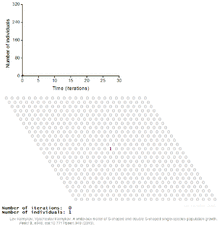
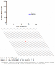
Individual-based models
Cellular automata are used to investigate mechanisms of population dynamics. Here are relatively simple models with one and two species.
Fisheries and wildlife management
In fisheries and wildlife management, population is affected by three dynamic rate functions.
- Natality or birth rate, often recruitment, which means reaching a certain size or reproductive stage. Usually refers to the age a fish can be caught and counted in nets.
- Population growth rate, which measures the growth of individuals in size and length. More important in fisheries, where population is often measured in biomass.
- Mortality, which includes harvest mortality and natural mortality. Natural mortality includes non-human predation, disease and old age.
If N1 is the number of individuals at time 1 then

where N0 is the number of individuals at time 0, B is the number of individuals born, D the number that died, I the number that immigrated, and E the number that emigrated between time 0 and time 1.
If we measure these rates over many time intervals, we can determine how a population's density changes over time. Immigration and emigration are present, but are usually not measured.
All of these are measured to determine the harvestable surplus, which is the number of individuals that can be harvested from a population without affecting long-term population stability or average population size. The harvest within the harvestable surplus is termed "compensatory" mortality, where the harvest deaths are substituted for the deaths that would have occurred naturally. Harvest above that level is termed "additive" mortality, because it adds to the number of deaths that would have occurred naturally. These terms are not necessarily judged as "good" and "bad," respectively, in population management. For example, a fish & game agency might aim to reduce the size of a deer population through additive mortality. Bucks might be targeted to increase buck competition, or does might be targeted to reduce reproduction and thus overall population size.
For the management of many fish and other wildlife populations, the goal is often to achieve the largest possible long-run sustainable harvest, also known as maximum sustainable yield (or MSY). Given a population dynamic model, such as any of the ones above, it is possible to calculate the population size that produces the largest harvestable surplus at equilibrium.[4] While the use of population dynamic models along with statistics and optimization to set harvest limits for fish and game is controversial among scientists,[5] it has been shown to be more effective than the use of human judgment in computer experiments where both incorrect models and natural resource management students competed to maximize yield in two hypothetical fisheries.[6][7] To give an example of a non-intuitive result, fisheries produce more fish when there is a nearby refuge from human predation in the form of a nature reserve, resulting in higher catches than if the whole area was open to fishing.[8][9]
For control applications
Population dynamics have been widely used in several control theory applications. With the use of evolutionary game theory, population games are broadly implemented for different industrial and daily-life contexts. Mostly used in multiple-input-multiple-output (MIMO) systems, although they can be adapted for use in single-input-single-output (SISO) systems. Some examples of applications are military campaigns, resource allocation for water distribution, dispatch of distributed generators, lab experiments, transport problems, communication problems, among others. Furthermore, with the adequate contextualization of industrial problems, population dynamics can be an efficient and easy-to-implement solution for control-related problems. Multiple academic research has been and is continuously carried out.
See also
- Delayed density dependence
- Holocene extinction
- Lotka-Volterra equations
- Minimum viable population
- Maximum sustainable yield
- Nicholson–Bailey model
- Overshoot (population)
- Pest insect population dynamics
- Population cycle
- Population dynamics of fisheries
- Population ecology
- Population genetics
- Population modeling
- Ricker model
- r/K selection theory
- Sigmoid curve
- Societal collapse
- System dynamics
References
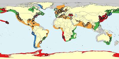
- ↑ Brotz, Lucas; Cheung, William W. L; Kleisner, Kristin; Pakhomov, Evgeny; Pauly, Daniel (2012). "Increasing jellyfish populations: Trends in Large Marine Ecosystems". Hydrobiologia. 690 (1): 3–20. doi:10.1007/s10750-012-1039-7.
- ↑ Jahn, Gary C; Almazan, Liberty P; Pacia, Jocelyn B (2005). "Effect of Nitrogen Fertilizer on the Intrinsic Rate of Increase of Hysteroneura setariae(Thomas) (Homoptera: Aphididae) on Rice (Oryza sativaL.)". Environmental Entomology. 34 (4): 938–43. doi:10.1603/0046-225X-34.4.938.
- 1 2 3 4 5 6 Yang, Louie. Population Dynamics. Davis: UC Davis, 2014.
- ↑ Clark, Colin (1990). Mathematical bioeconomics : the optimal management of renewable resources. New York: Wiley. ISBN 0471508837.
- ↑ Finley, C; Oreskes, N (2013). "Maximum sustained yield: A policy disguised as science". ICES Journal of Marine Science. 70 (2): 245–50. doi:10.1093/icesjms/fss192.
- ↑ Holden, Matthew H; Ellner, Stephen P (2016). "Human judgment vs. Quantitative models for the management of ecological resources". Ecological Applications. 26 (5): 1553–1565. doi:10.1890/15-1295. PMID 27755756.
- ↑ Standard, Pacific (2016-03-11). "Sometimes, Even Bad Models Make Better Decisions Than People". Pacific Standard. Retrieved 2017-01-28.
- ↑ Chakraborty, Kunal; Das, Kunal; Kar, T. K (2013). "An ecological perspective on marine reserves in prey–predator dynamics". Journal of Biological Physics. 39 (4): 749–76. doi:10.1007/s10867-013-9329-5. PMC 3758828. PMID 23949368.
- ↑ Lv, Yunfei; Yuan, Rong; Pei, Yongzhen (2013). "A prey-predator model with harvesting for fishery resource with reserve area". Applied Mathematical Modelling. 37 (5): 3048–62. doi:10.1016/j.apm.2012.07.030.
Further reading
- Andrey Korotayev, Artemy Malkov, and Daria Khaltourina. Introduction to Social Macrodynamics: Compact Macromodels of the World System Growth. ISBN 5-484-00414-4
- Turchin, P. 2003. Complex Population Dynamics: a Theoretical/Empirical Synthesis. Princeton, NJ: Princeton University Press.
- Weiss, Volkmar (2007). "The Population Cycle Drives Human History - from a Eugenic Phase into a Dysgenic Phase and Eventual Collapse". The Journal of Social, Political and Economic Studies. 32 (3): 327–58.
External links
- The Virtual Handbook on Population Dynamics. An online compilation of state-ot-the-art basic tools for the analysis of population dynamics with emphasis on benthic invertebrates.
| General |  | |
|---|---|---|
| Causes | ||
| Effects |
| |
| Mitigation | ||
| ||
| Major topics | |
|---|---|
| Biological and related topics | |
| Human impact on the environment | |
| Literature |
|
| Publications | |
| Lists | |
Events and organizations | |
| Related topics | |
| |