Student's t-distribution
In probability and statistics, Student's t-distribution (or simply the t-distribution) is any member of a family of continuous probability distributions that arises when estimating the mean of a normally distributed population in situations where the sample size is small and the population standard deviation is unknown. It was developed by William Sealy Gosset under the pseudonym Student.
|
Probability density function 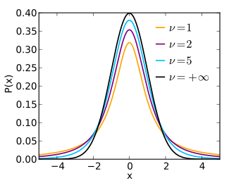 | |||
|
Cumulative distribution function  | |||
| Parameters | degrees of freedom (real) | ||
|---|---|---|---|
| Support | |||
| CDF |
| ||
| Mean | 0 for , otherwise undefined | ||
| Median | 0 | ||
| Mode | 0 | ||
| Variance | for , ∞ for , otherwise undefined | ||
| Skewness | 0 for , otherwise undefined | ||
| Ex. kurtosis | for , ∞ for , otherwise undefined | ||
| Entropy |
| ||
| MGF | undefined | ||
| CF |
for | ||


The t-distribution plays a role in a number of widely used statistical analyses, including Student's t-test for assessing the statistical significance of the difference between two sample means, the construction of confidence intervals for the difference between two population means, and in linear regression analysis. The Student's t-distribution also arises in the Bayesian analysis of data from a normal family.
If we take a sample of observations from a normal distribution, then the t-distribution with degrees of freedom can be defined as the distribution of the location of the sample mean relative to the true mean, divided by the sample standard deviation, after multiplying by the standardizing term . In this way, the t-distribution can be used to construct a confidence interval for the true mean.


The t-distribution is symmetric and bell-shaped, like the normal distribution, but has heavier tails, meaning that it is more prone to producing values that fall far from its mean. This makes it useful for understanding the statistical behavior of certain types of ratios of random quantities, in which variation in the denominator is amplified and may produce outlying values when the denominator of the ratio falls close to zero. The Student's t-distribution is a special case of the generalised hyperbolic distribution.
History and etymology
In statistics, the t-distribution was first derived as a posterior distribution in 1876 by Helmert[2][3][4] and Lüroth.[5][6][7] The t-distribution also appeared in a more general form as Pearson Type IV distribution in Karl Pearson's 1895 paper.[8]
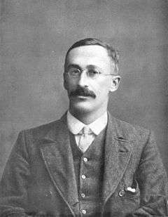
In the English-language literature the distribution takes its name from William Sealy Gosset's 1908 paper in Biometrika under the pseudonym "Student".[9] Gosset worked at the Guinness Brewery in Dublin, Ireland, and was interested in the problems of small samples – for example, the chemical properties of barley where sample sizes might be as few as 3. One version of the origin of the pseudonym is that Gosset's employer preferred staff to use pen names when publishing scientific papers instead of their real name, so he used the name "Student" to hide his identity. Another version is that Guinness did not want their competitors to know that they were using the t-test to determine the quality of raw material.[10][11]
Gosset's paper refers to the distribution as the "frequency distribution of standard deviations of samples drawn from a normal population". It became well known through the work of Ronald Fisher, who called the distribution "Student's distribution" and represented the test value with the letter t.[12][13]
How Student's distribution arises from sampling
Let be independently and identically drawn from the distribution , i.e. this is a sample of size from a normally distributed population with expected mean value and variance .


Let

be the sample mean and let

be the (Bessel-corrected) sample variance. Then the random variable

has a standard normal distribution (i.e. normal with expected mean 0 and variance 1), and the random variable

where has been substituted for , has a Student's t-distribution with degrees of freedom. The numerator and the denominator in the preceding expression are independent random variables despite being based on the same sample .


Definition
Probability density function
Student's t-distribution has the probability density function given by

where is the number of degrees of freedom and is the gamma function. This may also be written as


where B is the Beta function. In particular for integer valued degrees of freedom we have:
For even,

For odd,

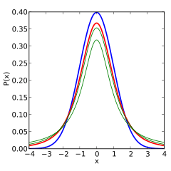
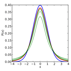
The probability density function is symmetric, and its overall shape resembles the bell shape of a normally distributed variable with mean 0 and variance 1, except that it is a bit lower and wider. As the number of degrees of freedom grows, the t-distribution approaches the normal distribution with mean 0 and variance 1. For this reason is also known as the normality parameter.[14]

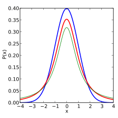
The following images show the density of the t-distribution for increasing values of . The normal distribution is shown as a blue line for comparison. Note that the t-distribution (red line) becomes closer to the normal distribution as increases.
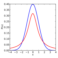 1 degree of freedom |
 2 degrees of freedom |
 3 degrees of freedom |
 5 degrees of freedom |
 10 degrees of freedom |
 30 degrees of freedom |
Cumulative distribution function
The cumulative distribution function can be written in terms of I, the regularized incomplete beta function. For t > 0,[15]

where

Other values would be obtained by symmetry. An alternative formula, valid for , is[15]


where 2F1 is a particular case of the hypergeometric function.
For information on its inverse cumulative distribution function, see quantile function § Student's t-distribution.
Special cases
Certain values of give an especially simple form.

- Distribution function:

- Density function:


- Distribution function:

- Density function:


- Distribution function:

- Density function:


- Distribution function:

- Density function:


- Distribution function:

- Density function:


- Distribution function:

- See Error function
- Density function:

How the t-distribution arises
Sampling distribution
Let be the numbers observed in a sample from a continuously distributed population with expected value . The sample mean and sample variance are given by:


The resulting t-value is

The t-distribution with degrees of freedom is the sampling distribution of the t-value when the samples consist of independent identically distributed observations from a normally distributed population. Thus for inference purposes t is a useful "pivotal quantity" in the case when the mean and variance are unknown population parameters, in the sense that the t-value has then a probability distribution that depends on neither nor .

Bayesian inference
In Bayesian statistics, a (scaled, shifted) t-distribution arises as the marginal distribution of the unknown mean of a normal distribution, when the dependence on an unknown variance has been marginalized out:[16]

where stands for the data , and represents any other information that may have been used to create the model. The distribution is thus the compounding of the conditional distribution of given the data and with the marginal distribution of given the data.


With data points, if uninformative, or flat, location and scale priors and can be taken for μ and σ2, then Bayes' theorem gives


a normal distribution and a scaled inverse chi-squared distribution respectively, where and

The marginalization integral thus becomes

This can be evaluated by substituting , where , giving


so

But the z integral is now a standard Gamma integral, which evaluates to a constant, leaving

This is a form of the t-distribution with an explicit scaling and shifting that will be explored in more detail in a further section below. It can be related to the standardized t-distribution by the substitution

The derivation above has been presented for the case of uninformative priors for and ; but it will be apparent that any priors that lead to a normal distribution being compounded with a scaled inverse chi-squared distribution will lead to a t-distribution with scaling and shifting for , although the scaling parameter corresponding to above will then be influenced both by the prior information and the data, rather than just by the data as above.


Characterization
As the distribution of a test statistic
Student's t-distribution with degrees of freedom can be defined as the distribution of the random variable T with[15][17]

where
- Z is a standard normal with expected value 0 and variance 1;
- V has a chi-squared distribution with degrees of freedom;
- Z and V are independent.
A different distribution is defined as that of the random variable defined, for a given constant μ, by

This random variable has a noncentral t-distribution with noncentrality parameter μ. This distribution is important in studies of the power of Student's t-test.
Derivation
Suppose X1, ..., Xn are independent realizations of the normally-distributed, random variable X, which has an expected value μ and variance σ2. Let

be the sample mean, and

be an unbiased estimate of the variance from the sample. It can be shown that the random variable

has a chi-squared distribution with degrees of freedom (by Cochran's theorem).[18] It is readily shown that the quantity

is normally distributed with mean 0 and variance 1, since the sample mean is normally distributed with mean μ and variance σ2/n. Moreover, it is possible to show that these two random variables (the normally distributed one Z and the chi-squared-distributed one V) are independent. Consequently the pivotal quantity


which differs from Z in that the exact standard deviation σ is replaced by the random variable Sn, has a Student's t-distribution as defined above. Notice that the unknown population variance σ2 does not appear in T, since it was in both the numerator and the denominator, so it canceled. Gosset intuitively obtained the probability density function stated above, with equal to n − 1, and Fisher proved it in 1925.[12]
The distribution of the test statistic T depends on , but not μ or σ; the lack of dependence on μ and σ is what makes the t-distribution important in both theory and practice.
As a maximum entropy distribution
Student's t-distribution is the maximum entropy probability distribution for a random variate X for which is fixed.[19]

Properties
Moments
For , the raw moments of the t-distribution are

Moments of order or higher do not exist.[20]
The term for , k even, may be simplified using the properties of the gamma function to


For a t-distribution with degrees of freedom, the expected value is 0 if , and its variance is if . The skewness is 0 if and the excess kurtosis is if .


Monte Carlo sampling
There are various approaches to constructing random samples from the Student's t-distribution. The matter depends on whether the samples are required on a stand-alone basis, or are to be constructed by application of a quantile function to uniform samples; e.g., in the multi-dimensional applications basis of copula-dependency. In the case of stand-alone sampling, an extension of the Box–Muller method and its polar form is easily deployed.[21] It has the merit that it applies equally well to all real positive degrees of freedom, ν, while many other candidate methods fail if ν is close to zero.[21]
Integral of Student's probability density function and p-value
The function A(t | ν) is the integral of Student's probability density function, f(t) between −t and t, for t ≥ 0. It thus gives the probability that a value of t less than that calculated from observed data would occur by chance. Therefore, the function A(t | ν) can be used when testing whether the difference between the means of two sets of data is statistically significant, by calculating the corresponding value of t and the probability of its occurrence if the two sets of data were drawn from the same population. This is used in a variety of situations, particularly in t-tests. For the statistic t, with ν degrees of freedom, A(t | ν) is the probability that t would be less than the observed value if the two means were the same (provided that the smaller mean is subtracted from the larger, so that t ≥ 0). It can be easily calculated from the cumulative distribution function Fν(t) of the t-distribution:

where Ix is the regularized incomplete beta function (a, b).
For statistical hypothesis testing this function is used to construct the p-value.
Generalized Student's t-distribution
In terms of scaling parameter or


Student's t distribution can be generalized to a three parameter location-scale family, introducing a location parameter and a scale parameter , through the relation


or

This means that has a classic Student's t distribution with degrees of freedom.

The resulting non-standardized Student's t-distribution has a density defined by:[22]

Here, does not correspond to a standard deviation: it is not the standard deviation of the scaled t distribution, which may not even exist; nor is it the standard deviation of the underlying normal distribution, which is unknown. simply sets the overall scaling of the distribution. In the Bayesian derivation of the marginal distribution of an unknown normal mean above, as used here corresponds to the quantity , where

- .

Equivalently, the distribution can be written in terms of , the square of this scale parameter:

Other properties of this version of the distribution are:[22]

This distribution results from compounding a Gaussian distribution (normal distribution) with mean and unknown variance, with an inverse gamma distribution placed over the variance with parameters and . In other words, the random variable X is assumed to have a Gaussian distribution with an unknown variance distributed as inverse gamma, and then the variance is marginalized out (integrated out). The reason for the usefulness of this characterization is that the inverse gamma distribution is the conjugate prior distribution of the variance of a Gaussian distribution. As a result, the non-standardized Student's t-distribution arises naturally in many Bayesian inference problems. See below.


Equivalently, this distribution results from compounding a Gaussian distribution with a scaled-inverse-chi-squared distribution with parameters and . The scaled-inverse-chi-squared distribution is exactly the same distribution as the inverse gamma distribution, but with a different parameterization, i.e. .

In terms of inverse scaling parameter λ
An alternative parameterization in terms of an inverse scaling parameter (analogous to the way precision is the reciprocal of variance), defined by the relation . The density is then given by:[23]


Other properties of this version of the distribution are:[23]

This distribution results from compounding a Gaussian distribution with mean and unknown precision (the reciprocal of the variance), with a gamma distribution placed over the precision with parameters and . In other words, the random variable X is assumed to have a normal distribution with an unknown precision distributed as gamma, and then this is marginalized over the gamma distribution.

Related distributions
- If has a Student's t-distribution with degree of freedom then X2 has an F-distribution:
- The noncentral t-distribution generalizes the t-distribution to include a location parameter. Unlike the nonstandardized t-distributions, the noncentral distributions are not symmetric (the median is not the same as the mode).
- The discrete Student's t-distribution is defined by its probability mass function at r being proportional to:[24]


- Here a, b, and k are parameters. This distribution arises from the construction of a system of discrete distributions similar to that of the Pearson distributions for continuous distributions.[25]

- One can generate Student-t samples by taking the ratio of variables from the normal distribution and the square-root of χ2-distribution. If we use instead of the normal distribution, e.g., the Irwin–Hall distribution, we obtain over-all a symmetric 4-parameter distribution, which includes the normal, the uniform, the triangular, the Student-t and the Cauchy distribution. This is also more flexible than some other symmetric generalizations of the normal distribution.
- t-distribution is an instance of ratio distributions
Uses
In frequentist statistical inference
Student's t-distribution arises in a variety of statistical estimation problems where the goal is to estimate an unknown parameter, such as a mean value, in a setting where the data are observed with additive errors. If (as in nearly all practical statistical work) the population standard deviation of these errors is unknown and has to be estimated from the data, the t-distribution is often used to account for the extra uncertainty that results from this estimation. In most such problems, if the standard deviation of the errors were known, a normal distribution would be used instead of the t-distribution.
Confidence intervals and hypothesis tests are two statistical procedures in which the quantiles of the sampling distribution of a particular statistic (e.g. the standard score) are required. In any situation where this statistic is a linear function of the data, divided by the usual estimate of the standard deviation, the resulting quantity can be rescaled and centered to follow Student's t-distribution. Statistical analyses involving means, weighted means, and regression coefficients all lead to statistics having this form.
Quite often, textbook problems will treat the population standard deviation as if it were known and thereby avoid the need to use the Student's t-distribution. These problems are generally of two kinds: (1) those in which the sample size is so large that one may treat a data-based estimate of the variance as if it were certain, and (2) those that illustrate mathematical reasoning, in which the problem of estimating the standard deviation is temporarily ignored because that is not the point that the author or instructor is then explaining.
Hypothesis testing
A number of statistics can be shown to have t-distributions for samples of moderate size under null hypotheses that are of interest, so that the t-distribution forms the basis for significance tests. For example, the distribution of Spearman's rank correlation coefficient ρ, in the null case (zero correlation) is well approximated by the t distribution for sample sizes above about 20.
Confidence intervals
Suppose the number A is so chosen that

when T has a t-distribution with n − 1 degrees of freedom. By symmetry, this is the same as saying that A satisfies

so A is the "95th percentile" of this probability distribution, or . Then


and this is equivalent to

Therefore, the interval whose endpoints are

is a 90% confidence interval for μ. Therefore, if we find the mean of a set of observations that we can reasonably expect to have a normal distribution, we can use the t-distribution to examine whether the confidence limits on that mean include some theoretically predicted value – such as the value predicted on a null hypothesis.
It is this result that is used in the Student's t-tests: since the difference between the means of samples from two normal distributions is itself distributed normally, the t-distribution can be used to examine whether that difference can reasonably be supposed to be zero.
If the data are normally distributed, the one-sided (1 − α)-upper confidence limit (UCL) of the mean, can be calculated using the following equation:

The resulting UCL will be the greatest average value that will occur for a given confidence interval and population size. In other words, being the mean of the set of observations, the probability that the mean of the distribution is inferior to UCL1−α is equal to the confidence level 1 − α.
Prediction intervals
The t-distribution can be used to construct a prediction interval for an unobserved sample from a normal distribution with unknown mean and variance.
In Bayesian statistics
The Student's t-distribution, especially in its three-parameter (location-scale) version, arises frequently in Bayesian statistics as a result of its connection with the normal distribution. Whenever the variance of a normally distributed random variable is unknown and a conjugate prior placed over it that follows an inverse gamma distribution, the resulting marginal distribution of the variable will follow a Student's t-distribution. Equivalent constructions with the same results involve a conjugate scaled-inverse-chi-squared distribution over the variance, or a conjugate gamma distribution over the precision. If an improper prior proportional to σ−2 is placed over the variance, the t-distribution also arises. This is the case regardless of whether the mean of the normally distributed variable is known, is unknown distributed according to a conjugate normally distributed prior, or is unknown distributed according to an improper constant prior.
Related situations that also produce a t-distribution are:
- The marginal posterior distribution of the unknown mean of a normally distributed variable, with unknown prior mean and variance following the above model.
- The prior predictive distribution and posterior predictive distribution of a new normally distributed data point when a series of independent identically distributed normally distributed data points have been observed, with prior mean and variance as in the above model.
Robust parametric modeling
The t-distribution is often used as an alternative to the normal distribution as a model for data, which often has heavier tails than the normal distribution allows for; see e.g. Lange et al.[26] The classical approach was to identify outliers and exclude or downweight them in some way. However, it is not always easy to identify outliers (especially in high dimensions), and the t-distribution is a natural choice of model for such data and provides a parametric approach to robust statistics.
A Bayesian account can be found in Gelman et al.[27] The degrees of freedom parameter controls the kurtosis of the distribution and is correlated with the scale parameter. The likelihood can have multiple local maxima and, as such, it is often necessary to fix the degrees of freedom at a fairly low value and estimate the other parameters taking this as given. Some authors report that values between 3 and 9 are often good choices. Venables and Ripley suggest that a value of 5 is often a good choice.
Student's t-process
For practical regression and prediction needs, Student's t-processes were introduced, that are generalisations of the Student t-distributions for functions. A Student's t-process is constructed from the Student t-distributions like a Gaussian process is constructed from the Gaussian distributions. For a Gaussian process, all sets of values have a multidimensional Gaussian distribution. Analogiusly, is a Student t-process on an interval if the correspondent values of the process () have a joint multivariate Student t-distribution.[28] These processes are used for regression, prediction, Bayesian optimization and related problems. For multivariate regression and multi-output prediction, the matrix-values Student's t-processes are introduced and used.[29]


Table of selected values
The following table lists values for t-distributions with ν degrees of freedom for a range of one-sided or two-sided critical regions. The first column is ν, the percentages along the top are confidence levels, and the numbers in the body of the table are the factors described in the section on confidence intervals.

Note that the last row with infinite ν gives critical points for a normal distribution since a t-distribution with infinitely many degrees of freedom is a normal distribution. (See Related distributions above).
| One-sided | 75% | 80% | 85% | 90% | 95% | 97.5% | 99% | 99.5% | 99.75% | 99.9% | 99.95% |
|---|---|---|---|---|---|---|---|---|---|---|---|
| Two-sided | 50% | 60% | 70% | 80% | 90% | 95% | 98% | 99% | 99.5% | 99.8% | 99.9% |
| 1 | 1.000 | 1.376 | 1.963 | 3.078 | 6.314 | 12.71 | 31.82 | 63.66 | 127.3 | 318.3 | 636.6 |
| 2 | 0.816 | 1.080 | 1.386 | 1.886 | 2.920 | 4.303 | 6.965 | 9.925 | 14.09 | 22.33 | 31.60 |
| 3 | 0.765 | 0.978 | 1.250 | 1.638 | 2.353 | 3.182 | 4.541 | 5.841 | 7.453 | 10.21 | 12.92 |
| 4 | 0.741 | 0.941 | 1.190 | 1.533 | 2.132 | 2.776 | 3.747 | 4.604 | 5.598 | 7.173 | 8.610 |
| 5 | 0.727 | 0.920 | 1.156 | 1.476 | 2.015 | 2.571 | 3.365 | 4.032 | 4.773 | 5.893 | 6.869 |
| 6 | 0.718 | 0.906 | 1.134 | 1.440 | 1.943 | 2.447 | 3.143 | 3.707 | 4.317 | 5.208 | 5.959 |
| 7 | 0.711 | 0.896 | 1.119 | 1.415 | 1.895 | 2.365 | 2.998 | 3.499 | 4.029 | 4.785 | 5.408 |
| 8 | 0.706 | 0.889 | 1.108 | 1.397 | 1.860 | 2.306 | 2.896 | 3.355 | 3.833 | 4.501 | 5.041 |
| 9 | 0.703 | 0.883 | 1.100 | 1.383 | 1.833 | 2.262 | 2.821 | 3.250 | 3.690 | 4.297 | 4.781 |
| 10 | 0.700 | 0.879 | 1.093 | 1.372 | 1.812 | 2.228 | 2.764 | 3.169 | 3.581 | 4.144 | 4.587 |
| 11 | 0.697 | 0.876 | 1.088 | 1.363 | 1.796 | 2.201 | 2.718 | 3.106 | 3.497 | 4.025 | 4.437 |
| 12 | 0.695 | 0.873 | 1.083 | 1.356 | 1.782 | 2.179 | 2.681 | 3.055 | 3.428 | 3.930 | 4.318 |
| 13 | 0.694 | 0.870 | 1.079 | 1.350 | 1.771 | 2.160 | 2.650 | 3.012 | 3.372 | 3.852 | 4.221 |
| 14 | 0.692 | 0.868 | 1.076 | 1.345 | 1.761 | 2.145 | 2.624 | 2.977 | 3.326 | 3.787 | 4.140 |
| 15 | 0.691 | 0.866 | 1.074 | 1.341 | 1.753 | 2.131 | 2.602 | 2.947 | 3.286 | 3.733 | 4.073 |
| 16 | 0.690 | 0.865 | 1.071 | 1.337 | 1.746 | 2.120 | 2.583 | 2.921 | 3.252 | 3.686 | 4.015 |
| 17 | 0.689 | 0.863 | 1.069 | 1.333 | 1.740 | 2.110 | 2.567 | 2.898 | 3.222 | 3.646 | 3.965 |
| 18 | 0.688 | 0.862 | 1.067 | 1.330 | 1.734 | 2.101 | 2.552 | 2.878 | 3.197 | 3.610 | 3.922 |
| 19 | 0.688 | 0.861 | 1.066 | 1.328 | 1.729 | 2.093 | 2.539 | 2.861 | 3.174 | 3.579 | 3.883 |
| 20 | 0.687 | 0.860 | 1.064 | 1.325 | 1.725 | 2.086 | 2.528 | 2.845 | 3.153 | 3.552 | 3.850 |
| 21 | 0.686 | 0.859 | 1.063 | 1.323 | 1.721 | 2.080 | 2.518 | 2.831 | 3.135 | 3.527 | 3.819 |
| 22 | 0.686 | 0.858 | 1.061 | 1.321 | 1.717 | 2.074 | 2.508 | 2.819 | 3.119 | 3.505 | 3.792 |
| 23 | 0.685 | 0.858 | 1.060 | 1.319 | 1.714 | 2.069 | 2.500 | 2.807 | 3.104 | 3.485 | 3.767 |
| 24 | 0.685 | 0.857 | 1.059 | 1.318 | 1.711 | 2.064 | 2.492 | 2.797 | 3.091 | 3.467 | 3.745 |
| 25 | 0.684 | 0.856 | 1.058 | 1.316 | 1.708 | 2.060 | 2.485 | 2.787 | 3.078 | 3.450 | 3.725 |
| 26 | 0.684 | 0.856 | 1.058 | 1.315 | 1.706 | 2.056 | 2.479 | 2.779 | 3.067 | 3.435 | 3.707 |
| 27 | 0.684 | 0.855 | 1.057 | 1.314 | 1.703 | 2.052 | 2.473 | 2.771 | 3.057 | 3.421 | 3.690 |
| 28 | 0.683 | 0.855 | 1.056 | 1.313 | 1.701 | 2.048 | 2.467 | 2.763 | 3.047 | 3.408 | 3.674 |
| 29 | 0.683 | 0.854 | 1.055 | 1.311 | 1.699 | 2.045 | 2.462 | 2.756 | 3.038 | 3.396 | 3.659 |
| 30 | 0.683 | 0.854 | 1.055 | 1.310 | 1.697 | 2.042 | 2.457 | 2.750 | 3.030 | 3.385 | 3.646 |
| 40 | 0.681 | 0.851 | 1.050 | 1.303 | 1.684 | 2.021 | 2.423 | 2.704 | 2.971 | 3.307 | 3.551 |
| 50 | 0.679 | 0.849 | 1.047 | 1.299 | 1.676 | 2.009 | 2.403 | 2.678 | 2.937 | 3.261 | 3.496 |
| 60 | 0.679 | 0.848 | 1.045 | 1.296 | 1.671 | 2.000 | 2.390 | 2.660 | 2.915 | 3.232 | 3.460 |
| 80 | 0.678 | 0.846 | 1.043 | 1.292 | 1.664 | 1.990 | 2.374 | 2.639 | 2.887 | 3.195 | 3.416 |
| 100 | 0.677 | 0.845 | 1.042 | 1.290 | 1.660 | 1.984 | 2.364 | 2.626 | 2.871 | 3.174 | 3.390 |
| 120 | 0.677 | 0.845 | 1.041 | 1.289 | 1.658 | 1.980 | 2.358 | 2.617 | 2.860 | 3.160 | 3.373 |
| ∞ | 0.674 | 0.842 | 1.036 | 1.282 | 1.645 | 1.960 | 2.326 | 2.576 | 2.807 | 3.090 | 3.291 |
Calculating the confidence interval
Let's say we have a sample with size 11, sample mean 10, and sample variance 2. For 90% confidence with 10 degrees of freedom, the one-sided t-value from the table is 1.372. Then with confidence interval calculated from

we determine that with 90% confidence we have a true mean lying below

In other words, 90% of the times that an upper threshold is calculated by this method from particular samples, this upper threshold exceeds the true mean.
And with 90% confidence we have a true mean lying above

In other words, 90% of the times that a lower threshold is calculated by this method from particular samples, this lower threshold lies below the true mean.
So that at 80% confidence (calculated from 100% − 2 × (1 − 90%) = 80%), we have a true mean lying within the interval

Saying that 80% of the times that upper and lower thresholds are calculated by this method from a given sample, the true mean is both below the upper threshold and above the lower threshold is not the same as saying that there is an 80% probability that the true mean lies between a particular pair of upper and lower thresholds that have been calculated by this method; see confidence interval and prosecutor's fallacy.
Nowadays, statistical software, such as the R programming language, and functions available in many spreadsheet programs compute values of the t-distribution and its inverse without tables.
See also
- Chi-squared distribution
- F-distribution
- Gamma distribution
- Folded-t and half-t distributions
- Hotelling's T-squared distribution
- Multivariate Student distribution
- t-statistic
- Tau-distribution, for internally studentized residuals
- Wilks' lambda distribution
- Wishart distribution
Notes
- Hurst, Simon. The Characteristic Function of the Student-t Distribution, Financial Mathematics Research Report No. FMRR006-95, Statistics Research Report No. SRR044-95 Archived February 18, 2010, at the Wayback Machine
- Helmert FR (1875). "Über die Berechnung des wahrscheinlichen Fehlers aus einer endlichen Anzahl wahrer Beobachtungsfehler". Z. Math. U. Physik. 20: 300–3.
- Helmert FR (1876). "Über die Wahrscheinlichkeit der Potenzsummen der Beobachtungsfehler und uber einige damit in Zusammenhang stehende Fragen". Z. Math. Phys. 21: 192–218.
- Helmert FR (1876). "Die Genauigkeit der Formel von Peters zur Berechnung des wahrscheinlichen Beobachtungsfehlers directer Beobachtungen gleicher Genauigkeit" [The accuracy of Peters' formula for calculating the probable observation error of direct observations of the same accuracy] (PDF). Astron. Nachr. (in German). 88 (8–9): 113–132. Bibcode:1876AN.....88..113H. doi:10.1002/asna.18760880802.
- Lüroth J (1876). "Vergleichung von zwei Werten des wahrscheinlichen Fehlers". Astron. Nachr. 87 (14): 209–20. Bibcode:1876AN.....87..209L. doi:10.1002/asna.18760871402.
- Pfanzagl J, Sheynin O (1996). "Studies in the history of probability and statistics. XLIV. A forerunner of the t-distribution". Biometrika. 83 (4): 891–898. doi:10.1093/biomet/83.4.891. MR 1766040.
- Sheynin O (1995). "Helmert's work in the theory of errors". Arch. Hist. Exact Sci. 49 (1): 73–104. doi:10.1007/BF00374700.
- Pearson, K. (1895-01-01). "Contributions to the Mathematical Theory of Evolution. II. Skew Variation in Homogeneous Material". Philosophical Transactions of the Royal Society A: Mathematical, Physical and Engineering Sciences. 186: 343–414 (374). doi:10.1098/rsta.1895.0010. ISSN 1364-503X.
- "Student" [William Sealy Gosset] (1908). "The probable error of a mean" (PDF). Biometrika. 6 (1): 1–25. doi:10.1093/biomet/6.1.1. hdl:10338.dmlcz/143545. JSTOR 2331554.
- Wendl MC (2016). "Pseudonymous fame". Science. 351 (6280): 1406. doi:10.1126/science.351.6280.1406. PMID 27013722.
- Mortimer RG (2005). Mathematics for physical chemistry (3rd ed.). Burlington, MA: Elsevier. pp. 326. ISBN 9780080492889. OCLC 156200058.
- Fisher RA (1925). "Applications of "Student's" distribution" (PDF). Metron. 5: 90–104. Archived from the original (PDF) on 5 Mar 2016.
- Walpole RE, Myers R, Myers S, et al. (2006). Probability & Statistics for Engineers & Scientists (7th ed.). New Delhi: Pearson. p. 237. ISBN 9788177584042. OCLC 818811849.
- Kruschke JK (2015). Doing Bayesian Data Analysis (2nd ed.). Academic Press. ISBN 9780124058880. OCLC 959632184.
- Johnson NL, Kotz S, Balakrishnan N (1995). "Chapter 28". Continuous Univariate Distributions. 2 (2nd ed.). Wiley. ISBN 9780471584940.
- Gelman AB, Carlin JS, Rubin DB, et al. (1997). Bayesian Data Analysis (2nd ed.). Boca Raton: Chapman & Hall. p. 68. ISBN 9780412039911.
- Hogg RV, Craig AT (1978). Introduction to Mathematical Statistics (4th ed.). New York: Macmillan. ASIN B010WFO0SA. Sections 4.4 and 4.8
- Cochran WG (1934). "The distribution of quadratic forms in a normal system, with applications to the analysis of covariance". Math. Proc. Camb. Philos. Soc. 30 (2): 178–191. Bibcode:1934PCPS...30..178C. doi:10.1017/S0305004100016595.
- Park SY, Bera AK (2009). "Maximum entropy autoregressive conditional heteroskedasticity model". J. Econom. 150 (2): 219–230. doi:10.1016/j.jeconom.2008.12.014.
- Casella G, Berger RL (1990). Statistical Inference. Duxbury Resource Center. p. 56. ISBN 9780534119584.
- Bailey RW (1994). "Polar Generation of Random Variates with the t-Distribution". Math. Comput. 62 (206): 779–781. doi:10.2307/2153537. JSTOR 2153537.
- Jackman, S. (2009). Bayesian Analysis for the Social Sciences. Wiley. p. 507. doi:10.1002/9780470686621. ISBN 9780470011546.
- Bishop, C.M. (2006). Pattern Recognition and Machine Learning. New York, NY: Springer. ISBN 9780387310732.
- Ord JK (1972). Families of Frequency Distributions. London: Griffin. ISBN 9780852641378. See Table 5.1.
- Ord JK (1972). "Chapter 5". Families of frequency distributions. London: Griffin. ISBN 9780852641378.
- Lange KL, Little RJ, Taylor JM (1989). "Robust Statistical Modeling Using the t Distribution" (PDF). J. Am. Stat. Assoc. 84 (408): 881–896. doi:10.1080/01621459.1989.10478852. JSTOR 2290063.
- Gelman AB, Carlin JB, Stern HS, et al. (2014). "Computationally efficient Markov chain simulation". Bayesian Data Analysis. Boca Raton, FL: CRC Press. p. 293. ISBN 9781439898208.
- Shah, Amar; Wilson, Andrew Gordon; Ghahramani, Zoubin (2014). "Student t-processes as alternatives to Gaussian processes" (PDF). JMLR. 33 (Proceedings of the 17th International Conference on Artificial Intelligence and Statistics (AISTATS) 2014, Reykjavik, Iceland): 877–885.
- Chen, Zexun; Wang, Bo; Gorban, Alexander N. (2019). "Multivariate Gaussian and Student-t process regression for multi-output prediction". Neural Computing and Applications. arXiv:1703.04455. doi:10.1007/s00521-019-04687-8.
References
- Senn, S.; Richardson, W. (1994). "The first t-test". Statistics in Medicine. 13 (8): 785–803. doi:10.1002/sim.4780130802. PMID 8047737.
- Hogg RV, Craig AT (1978). Introduction to Mathematical Statistics (4th ed.). New York: Macmillan. ASIN B010WFO0SA.
- Venables, W. N.; Ripley, B. D. (2002). Modern Applied Statistics with S (Fourth ed.). Springer.
- Gelman, Andrew; John B. Carlin; Hal S. Stern; Donald B. Rubin (2003). Bayesian Data Analysis (Second Edition). CRC/Chapman & Hall. ISBN 1-58488-388-X.
External links
- Hazewinkel, Michiel, ed. (2001) [1994], "Student distribution", Encyclopedia of Mathematics, Springer Science+Business Media B.V. / Kluwer Academic Publishers, ISBN 978-1-55608-010-4
- Earliest Known Uses of Some of the Words of Mathematics (S) (Remarks on the history of the term "Student's distribution")
- Rouaud, M. (2013), Probability, Statistics and Estimation (PDF) (short ed.) First Students on page 112.