Gaussian process
In probability theory and statistics, a Gaussian process is a stochastic process (a collection of random variables indexed by time or space), such that every finite collection of those random variables has a multivariate normal distribution, i.e. every finite linear combination of them is normally distributed. The distribution of a Gaussian process is the joint distribution of all those (infinitely many) random variables, and as such, it is a distribution over functions with a continuous domain, e.g. time or space.
A machine-learning algorithm that involves a Gaussian process uses lazy learning and a measure of the similarity between points (the kernel function) to predict the value for an unseen point from training data. The prediction is not just an estimate for that point, but also has uncertainty information—it is a one-dimensional Gaussian distribution.[1] For multi-output predictions, multivariate Gaussian processes [2] are used, for which the multivariate Gaussian distribution is the marginal distribution at each point.
For some kernel functions, matrix algebra can be used to calculate the predictions using the technique of kriging. When a parameterised kernel is used, optimisation software is typically used to fit a Gaussian process model.
The concept of Gaussian processes is named after Carl Friedrich Gauss because it is based on the notion of the Gaussian distribution (normal distribution). Gaussian processes can be seen as an infinite-dimensional generalization of multivariate normal distributions.
Gaussian processes are useful in statistical modelling, benefiting from properties inherited from the normal distribution. For example, if a random process is modelled as a Gaussian process, the distributions of various derived quantities can be obtained explicitly. Such quantities include the average value of the process over a range of times and the error in estimating the average using sample values at a small set of times.
Definition
A time continuous stochastic process is Gaussian if and only if for every finite set of indices in the index set


is a multivariate Gaussian random variable.[3] That is the same as saying every linear combination of has a univariate normal (or Gaussian) distribution.

Using characteristic functions of random variables, the Gaussian property can be formulated as follows: is Gaussian if and only if, for every finite set of indices , there are real-valued , with such that the following equality holds for all


- .

where denotes the imaginary unit such that .


The numbers and can be shown to be the covariances and means of the variables in the process.[4]


Stationarity
For general stochastic processes strict-sense stationarity implies wide-sense stationarity but not every wide-sense stationary stochastic process is strict-sense stationary. However, for a Gaussian stochastic process the two concepts are equivalent.[5]:p. 518
A Gaussian stochastic process is strict-sense stationary if, and only if, it is wide-sense stationary.
Example
There is an explicit representation for stationary Gaussian processes.[6] A simple example of this representation is

where and are independent random variables with the standard normal distribution.


Covariance functions
A key fact of Gaussian processes is that they can be completely defined by their second-order statistics.[7] Thus, if a Gaussian process is assumed to have mean zero, defining the covariance function completely defines the process' behaviour. Importantly the non-negative definiteness of this function enables its spectral decomposition using the Karhunen–Loève expansion. Basic aspects that can be defined through the covariance function are the process' stationarity, isotropy, smoothness and periodicity.[8][9]
Stationarity refers to the process' behaviour regarding the separation of any two points and . If the process is stationary, it depends on their separation, , while if non-stationary it depends on the actual position of the points and . For example, the special case of an Ornstein–Uhlenbeck process, a Brownian motion process, is stationary.


If the process depends only on , the Euclidean distance (not the direction) between and , then the process is considered isotropic. A process that is concurrently stationary and isotropic is considered to be homogeneous;[10] in practice these properties reflect the differences (or rather the lack of them) in the behaviour of the process given the location of the observer.

Ultimately Gaussian processes translate as taking priors on functions and the smoothness of these priors can be induced by the covariance function.[8] If we expect that for "near-by" input points and their corresponding output points and to be "near-by" also, then the assumption of continuity is present. If we wish to allow for significant displacement then we might choose a rougher covariance function. Extreme examples of the behaviour is the Ornstein–Uhlenbeck covariance function and the squared exponential where the former is never differentiable and the latter infinitely differentiable.


Periodicity refers to inducing periodic patterns within the behaviour of the process. Formally, this is achieved by mapping the input to a two dimensional vector .

Usual covariance functions
There are a number of common covariance functions:[9]
- Constant :
- Linear:
- white Gaussian noise:
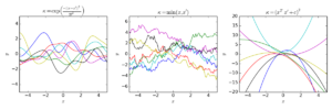
- Squared exponential:
- Ornstein–Uhlenbeck:
- Matérn:
- Periodic:
- Rational quadratic:


Here . The parameter is the characteristic length-scale of the process (practically, "how close" two points and have to be to influence each other significantly), is the Kronecker delta and the standard deviation of the noise fluctuations. Moreover, is the modified Bessel function of order and is the gamma function evaluated at . Importantly, a complicated covariance function can be defined as a linear combination of other simpler covariance functions in order to incorporate different insights about the data-set at hand.


Clearly, the inferential results are dependent on the values of the hyperparameters (e.g. and ) defining the model's behaviour. A popular choice for is to provide maximum a posteriori (MAP) estimates of it with some chosen prior. If the prior is very near uniform, this is the same as maximizing the marginal likelihood of the process; the marginalization being done over the observed process values .[9] This approach is also known as maximum likelihood II, evidence maximization, or empirical Bayes.[11]

Continuity
For a Gaussian process, continuity in probability is equivalent to mean-square continuity, [12]:145 and continuity with probability one is equivalent to sample continuity.[13]:91 "Gaussian processes are discontinuous at fixed points." The latter implies, but is not implied by, continuity in probability. Continuity in probability holds if and only if the mean and autocovariance are continuous functions. In contrast, sample continuity was challenging even for stationary Gaussian processes (as probably noted first by Andrey Kolmogorov), and more challenging for more general processes.[14]:Sect. 2.8 [15]:69,81 [16]:80 [17] As usual, by a sample continuous process one means a process that admits a sample continuous modification. [18]:292 [19]:424
Stationary case
For a stationary Gaussian process some conditions on its spectrum are sufficient for sample continuity, but fail to be necessary. A necessary and sufficient condition, sometimes called Dudley-Fernique theorem, involves the function defined by


(the right-hand side does not depend on due to stationarity). Continuity of in probability is equivalent to continuity of at When convergence of to (as ) is too slow, sample continuity of may fail. Convergence of the following integrals matters:


these two integrals being equal according to integration by substitution The first integrand need not be bounded as thus the integral may converge () or diverge (). Taking for example for large that is, for small one obtains when and when In these two cases the function is increasing on but generally it is not. Moreover, the condition


- there exists such that is monotone on


does not follow from continuity of and the evident relations (for all ) and


Theorem 1. Let be continuous and satisfy Then the condition is necessary and sufficient for sample continuity of


Some history.[19]:424 Sufficiency was announced by Xavier Fernique in 1964, but the first proof was published by Richard M. Dudley in 1967.[18]:Theorem 7.1 Necessity was proved by Michael B. Marcus and Lawrence Shepp in 1970.[20]:380
There exist sample continuous processes such that they violate condition An example found by Marcus and Shepp [20]:387 is a random lacunary Fourier series


where are independent random variables with standard normal distribution; frequencies are a fast growing sequence; and coefficients satisfy The latter relation implies whence almost surely, which ensures uniform convergence of the Fourier series almost surely, and sample continuity of


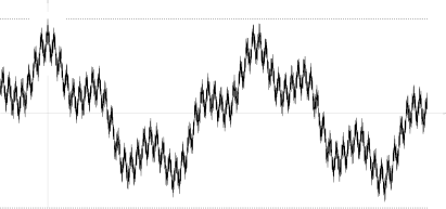
Its autocovariation function

is nowhere monotone (see the picture), as well as the corresponding function


Brownian motion as the integral of Gaussian processes
A Wiener process (aka Brownian motion) is the integral of a white noise generalized Gaussian process. It is not stationary, but it has stationary increments.
The Ornstein–Uhlenbeck process is a stationary Gaussian process.
The Brownian bridge is (like the Ornstein–Uhlenbeck process) an example of a Gaussian process whose increments are not independent.
The fractional Brownian motion is a Gaussian process whose covariance function is a generalisation of that of the Wiener process.
Driscoll's zero-one law
Driscoll's zero-one law is a result characterizing the sample functions generated by a Gaussian process.
Let be a mean-zero Gaussian process with non-negative definite covariance function . Let be a Reproducing kernel Hilbert space with positive definite kernel .


Then
- ,

where and are the covariance matrices of all possible pairs of points, implies


- .

What's more,

implies
- .[21]

This has significant implications when , as

- .

As such, almost all sample paths of a mean-zero Gaussian process with positive definite kernel will lie outside of the Hilbert space .

Applications
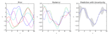
A Gaussian process can be used as a prior probability distribution over functions in Bayesian inference.[9][23] Given any set of N points in the desired domain of your functions, take a multivariate Gaussian whose covariance matrix parameter is the Gram matrix of your N points with some desired kernel, and sample from that Gaussian. For solution of the multi-output prediction problem, Gaussian process regression for vector-valued function was developed. In this method, a 'big' covariance is constructed, which describes the correlations between all the input and output variables taken in N points in the desired domain.[24] This approach was elaborated in detail for the matrix-valued Gaussian processes and generalised to processes with 'heavier tails' like Student-t processes.[2]
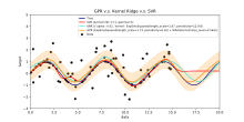
Inference of continuous values with a Gaussian process prior is known as Gaussian process regression, or kriging; extending Gaussian process regression to multiple target variables is known as cokriging.[25] Gaussian processes are thus useful as a powerful non-linear multivariate interpolation tool. Gaussian process regression can be further extended to address learning tasks in both supervised (e.g. probabilistic classification[9]) and unsupervised (e.g. manifold learning[7]) learning frameworks.
Gaussian processes can also be used in the context of mixture of experts models, for example.[26][27] The underlying rationale of such a learning framework consists in the assumption that a given mapping cannot be well captured by a single Gaussian process model. Instead, the observation space is divided into subsets, each of which is characterized by a different mapping function; each of these is learned via a different Gaussian process component in the postulated mixture.
Gaussian process prediction, or Kriging
When concerned with a general Gaussian process regression problem (Kriging), it is assumed that for a Gaussian process observed at coordinates , the vector of values is just one sample from a multivariate Gaussian distribution of dimension equal to number of observed coordinates . Therefore, under the assumption of a zero-mean distribution, , where is the covariance matrix between all possible pairs for a given set of hyperparameters θ.[9] As such the log marginal likelihood is:


and maximizing this marginal likelihood towards θ provides the complete specification of the Gaussian process f. One can briefly note at this point that the first term corresponds to a penalty term for a model's failure to fit observed values and the second term to a penalty term that increases proportionally to a model's complexity. Having specified θ making predictions about unobserved values at coordinates x* is then only a matter of drawing samples from the predictive distribution where the posterior mean estimate A is defined as


and the posterior variance estimate B is defined as:

where is the covariance between the new coordinate of estimation x* and all other observed coordinates x for a given hyperparameter vector θ, and are defined as before and is the variance at point x* as dictated by θ. It is important to note that practically the posterior mean estimate (the "point estimate") is just a linear combination of the observations ; in a similar manner the variance of is actually independent of the observations . A known bottleneck in Gaussian process prediction is that the computational complexity of prediction is cubic in the number of points |x| and as such can become unfeasible for larger data sets.[8] Works on sparse Gaussian processes, that usually are based on the idea of building a representative set for the given process f, try to circumvent this issue.[28][29]


Bayesian neural networks as Gaussian processes
Bayesian neural networks are a particular type of Bayesian network that results from treating deep learning and artificial neural network models probabilistically, and assigning a prior distribution to their parameters. Computation in artificial neural networks is usually organized into sequential layers of artificial neurons. The number of neurons in a layer is called the layer width. As layer width grows large, many Bayesian neural networks reduce to a Gaussian process with a closed form compositional kernel. This Gaussian process is called the Neural Network Gaussian Process (NNGP). It allows predictions from Bayesian neural networks to be more efficiently evaluated, and provides an analytic tool to understand deep learning models.
See also
- Bayes linear statistics
- Bayesian interpretation of regularization
- Kriging
- Gaussian free field
- Gradient-enhanced kriging (GEK)
- Student's t-process
References
- "Platypus Innovation: A Simple Intro to Gaussian Processes (a great data modelling tool)". 2016-05-10.
- Chen, Zexun; Wang, Bo; Gorban, Alexander N. (2019). "Multivariate Gaussian and Student-t process regression for multi-output prediction". Neural Computing and Applications. arXiv:1703.04455. doi:10.1007/s00521-019-04687-8.
- MacKay, David, J.C. (2003). Information Theory, Inference, and Learning Algorithms (PDF). Cambridge University Press. p. 540. ISBN 9780521642989.
The probability distribution of a function is a Gaussian processes if for any finite selection of points , the density is a Gaussian
- Dudley, R.M. (1989). Real Analysis and Probability. Wadsworth and Brooks/Cole.
- Amos Lapidoth (8 February 2017). A Foundation in Digital Communication. Cambridge University Press. ISBN 978-1-107-17732-1.
- Kac, M.; Siegert, A.J.F (1947). "An Explicit Representation of a Stationary Gaussian Process". The Annals of Mathematical Statistics. 18 (3): 438–442. doi:10.1214/aoms/1177730391.
- Bishop, C.M. (2006). Pattern Recognition and Machine Learning. Springer. ISBN 978-0-387-31073-2.
- Barber, David (2012). Bayesian Reasoning and Machine Learning. Cambridge University Press. ISBN 978-0-521-51814-7.
- Rasmussen, C.E.; Williams, C.K.I (2006). Gaussian Processes for Machine Learning. MIT Press. ISBN 978-0-262-18253-9.
- Grimmett, Geoffrey; David Stirzaker (2001). Probability and Random Processes. Oxford University Press. ISBN 978-0198572220.
- Seeger, Matthias (2004). "Gaussian Processes for Machine Learning". International Journal of Neural Systems. 14 (2): 69–104. CiteSeerX 10.1.1.71.1079. doi:10.1142/s0129065704001899. PMID 15112367.
- Dudley, R. M. (1975). "The Gaussian process and how to approach it" (PDF). Proceedings of the International Congress of Mathematicians. 2. pp. 143–146.
- Dudley, R. M. (1973). "Sample functions of the Gaussian process". Annals of Probability. 1 (1): 66–103. doi:10.1007/978-1-4419-5821-1_13. ISBN 978-1-4419-5820-4.
- Talagrand, Michel (2014). Upper and lower bounds for stochastic processes: modern methods and classical problems. Ergebnisse der Mathematik und ihrer Grenzgebiete. 3. Folge / A Series of Modern Surveys in Mathematics. Springer, Heidelberg. ISBN 978-3-642-54074-5.
- Ledoux, Michel (1994). "Isoperimetry and Gaussian analysis". Lecture Notes in Mathematics. 1648. Springer, Berlin. pp. 165–294. doi:10.1007/BFb0095676. ISBN 978-3-540-62055-6.
- Adler, Robert J. (1990). "An introduction to continuity, extrema, and related topics for general Gaussian processes". Lecture Notes-Monograph Series. Institute of Mathematical Statistics. 12: i–155. JSTOR 4355563.
- Berman, Simeon M. (1992). "Review of: Adler 1990 'An introduction to continuity...'". Mathematical Reviews. MR 1088478.
- Dudley, R. M. (1967). "The sizes of compact subsets of Hilbert space and continuity of Gaussian processes". Journal of Functional Analysis. 1 (3): 290–330. doi:10.1016/0022-1236(67)90017-1.
- Marcus, M.B.; Shepp, Lawrence A. (1972). "Sample behavior of Gaussian processes". Proceedings of the sixth Berkeley symposium on mathematical statistics and probability, vol. II: probability theory. Univ. California, Berkeley. pp. 423–441.
- Marcus, Michael B.; Shepp, Lawrence A. (1970). "Continuity of Gaussian processes". Transactions of the American Mathematical Society. 151 (2): 377–391. doi:10.1090/s0002-9947-1970-0264749-1. JSTOR 1995502.
- Driscoll, Michael F. (1973). "The reproducing kernel Hilbert space structure of the sample paths of a Gaussian process". Zeitschrift für Wahrscheinlichkeitstheorie und Verwandte Gebiete. 26 (4): 309–316. doi:10.1007/BF00534894. ISSN 0044-3719.
- The documentation for scikit-learn also has similar examples.
- Liu, W.; Principe, J.C.; Haykin, S. (2010). Kernel Adaptive Filtering: A Comprehensive Introduction. John Wiley. ISBN 978-0-470-44753-6. Archived from the original on 2016-03-04. Retrieved 2010-03-26.
- Álvarez, Mauricio A.; Rosasco, Lorenzo; Lawrence, Neil D. (2012). "Kernels for vector-valued functions: A review" (PDF). Foundations and Trends in Machine Learning. 4 (3): 195–266. doi:10.1561/2200000036.
- Stein, M.L. (1999). Interpolation of Spatial Data: Some Theory for Kriging. Springer.
- Platanios, Emmanouil A.; Chatzis, Sotirios P. (2014). "Gaussian Process-Mixture Conditional Heteroscedasticity". IEEE Transactions on Pattern Analysis and Machine Intelligence. 36 (5): 888–900. doi:10.1109/TPAMI.2013.183. PMID 26353224.
- Chatzis, Sotirios P. (2013). "A latent variable Gaussian process model with Pitman–Yor process priors for multiclass classification". Neurocomputing. 120: 482–489. doi:10.1016/j.neucom.2013.04.029.
- Smola, A.J.; Schoellkopf, B. (2000). "Sparse greedy matrix approximation for machine learning". Proceedings of the Seventeenth International Conference on Machine Learning: 911–918. CiteSeerX 10.1.1.43.3153.
- Csato, L.; Opper, M. (2002). "Sparse on-line Gaussian processes". Neural Computation. 14 (3): 641–668. CiteSeerX 10.1.1.335.9713. doi:10.1162/089976602317250933. PMID 11860686.


External links
- The Gaussian Processes Web Site, including the text of Rasmussen and Williams' Gaussian Processes for Machine Learning
- A gentle introduction to Gaussian processes
- A Review of Gaussian Random Fields and Correlation Functions
- Efficient Reinforcement Learning using Gaussian Processes
Software
- GPML: A comprehensive Matlab toolbox for GP regression and classification
- STK: a Small (Matlab/Octave) Toolbox for Kriging and GP modeling
- Kriging module in UQLab framework (Matlab)
- Matlab/Octave function for stationary Gaussian fields
- Yelp MOE – A black box optimization engine using Gaussian process learning
- ooDACE – A flexible object-oriented Kriging Matlab toolbox.
- GPstuff – Gaussian process toolbox for Matlab and Octave
- GPy – A Gaussian processes framework in Python
- GSTools - A geostatistical toolbox, including Gaussian process regression, written in Python
- Interactive Gaussian process regression demo
- Basic Gaussian process library written in C++11
- scikit-learn – A machine learning library for Python which includes Gaussian process regression and classification
- - The Kriging toolKit (KriKit) is developed at the Institute of Bio- and Geosciences 1 (IBG-1) of Forschungszentrum Jülich (FZJ)
Video tutorials
- Gaussian Process Basics by David MacKay
- Learning with Gaussian Processes by Carl Edward Rasmussen
- Bayesian inference and Gaussian processes by Carl Edward Rasmussen
| Authority control |
|
|---|