Density estimation
In probability and statistics, density estimation is the construction of an estimate, based on observed data, of an unobservable underlying probability density function. The unobservable density function is thought of as the density according to which a large population is distributed; the data are usually thought of as a random sample from that population.
A variety of approaches to density estimation are used, including Parzen windows and a range of data clustering techniques, including vector quantization. The most basic form of density estimation is a rescaled histogram.
Example of density estimation

We will consider records of the incidence of diabetes. The following is quoted verbatim from the data set description:
- A population of women who were at least 21 years old, of Pima Indian heritage and living near Phoenix, Arizona, was tested for diabetes mellitus according to World Health Organization criteria. The data were collected by the US National Institute of Diabetes and Digestive and Kidney Diseases. We used the 532 complete records.[1][2]
In this example, we construct three density estimates for "glu" (plasma glucose concentration), one conditional on the presence of diabetes, the second conditional on the absence of diabetes, and the third not conditional on diabetes. The conditional density estimates are then used to construct the probability of diabetes conditional on "glu".
The "glu" data were obtained from the MASS package[3] of the R programming language. Within R, ?Pima.tr and ?Pima.te give a fuller account of the data.
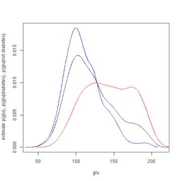
The mean of "glu" in the diabetes cases is 143.1 and the standard deviation is 31.26. The mean of "glu" in the non-diabetes cases is 110.0 and the standard deviation is 24.29. From this we see that, in this data set, diabetes cases are associated with greater levels of "glu". This will be made clearer by plots of the estimated density functions.
The first figure shows density estimates of p(glu | diabetes=1), p(glu | diabetes=0), and p(glu). The density estimates are kernel density estimates using a Gaussian kernel. That is, a Gaussian density function is placed at each data point, and the sum of the density functions is computed over the range of the data.
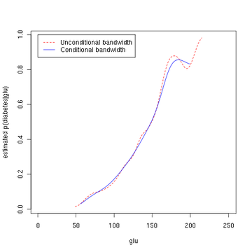
From the density of "glu" conditional on diabetes, we can obtain the probability of diabetes conditional on "glu" via Bayes' rule. For brevity, "diabetes" is abbreviated "db." in this formula.

The second figure shows the estimated posterior probability p(diabetes=1 | glu). From these data, it appears that an increased level of "glu" is associated with diabetes.
Script for example
The following R commands will create the figures shown above. These commands can be entered at the command prompt by using cut and paste.
library(MASS)
data(Pima.tr)
data(Pima.te)

Pima <- rbind (Pima.tr, Pima.te)
glu  <- Pima[, 'glu']

d0 <- Pima[, 'type'] == 'No'
d1 <- Pima[, 'type'] == 'Yes'
base.rate.d1 <- sum(d1) / (sum(d1) + sum(d0))

glu.density    <- density (glu)
glu.d0.density <- density (glu[d0])
glu.d1.density <- density (glu[d1])

glu.d0.f <- approxfun(glu.d0.density$x, glu.d0.density$y)
glu.d1.f <- approxfun(glu.d1.density$x, glu.d1.density$y)

p.d.given.glu <- function(glu, base.rate.d1)
{
    p1 <- glu.d1.f(glu) * base.rate.d1
    p0 <- glu.d0.f(glu) * (1 - base.rate.d1)
    p1 / (p0 + p1)
}

x <- 1:250
y <- p.d.given.glu (x, base.rate.d1)
plot(x, y, type='l', col='red', xlab='glu', ylab='estimated p(diabetes|glu)')

plot(density(glu[d0]), col='blue', xlab='glu', ylab='estimate p(glu),
     p(glu|diabetes), p(glu|not diabetes)', main=NA)
lines(density(glu[d1]), col='red')
Note that the above conditional density estimator uses bandwidths that are optimal for unconditional densities. Alternatively, one could use the method of Hall, Racine and Li (2004)[4] and the R np package[5]
for automatic (data-driven) bandwidth selection that is
optimal for conditional density estimates; see the np vignette[6] for an introduction to the np package. The following R commands use the npcdens() function to deliver optimal smoothing. Note that the response "Yes"/"No" is a factor.
library(np)

fy.x <- npcdens(type~glu, nmulti=1, data=Pima)

Pima.eval <- data.frame(type=factor("Yes"),
                        glu=seq(min(Pima$glu), max(Pima$glu), length=250))

plot(x, y, type='l', lty=2, col='red', xlab='glu',
     ylab='estimated p(diabetes|glu)')
lines(Pima.eval$glu, predict(fy.x, newdata=Pima.eval), col="blue")
legend(0, 1, c("Unconditional bandwidth", "Conditional bandwidth"),
       col=c("red", "blue"), lty=c(2, 1))
The third figure uses optimal smoothing via the method of Hall, Racine, and Li[4] indicating that the unconditional density bandwidth used in the second figure above yields a conditional density estimate that may be somewhat undersmoothed.
Application and Purpose
A very natural use of density estimates is in the informal investigation of the properties of a given set of data. Density estimates can give valuable indication of such features as skewness and multimodality in the data. In some cases they will yield conclusions that may then be regarded as self-evidently true, while in others all they will do is to point the way to further analysis and/or data collection.[7]
An important aspect of statistics is often the presentation of data back to the client in order to provide explanation and illustration of conclusions that may possibly have been obtained by other means. Density estimates are ideal for this purpose, for the simple reason that they are fairly easily comprehensible to non-mathematicians.
More examples illustrating the use of density estimates for exploratory and presentational purposes, including the important case of bivariate data.[9]
Density estimation is also frequently used in anomaly detection or novelty detection:[10] if an observation lies in a very low-density region, it is likely to be an anomaly or a novelty.
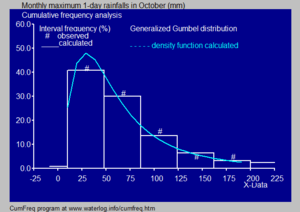
- In hydrology the histogram and estimated density function of rainfall and river discharge data, analysed with a probability distribution, are used to gain insight in their behaviour and frequency of occurrence.[11] An example is shown in the blue figure.
See also
References
- "Diabetes in Pima Indian Women - R documentation".
- Smith, J. W., Everhart, J. E., Dickson, W. C., Knowler, W. C. and Johannes, R. S. (1988). R. A. Greenes (ed.). "Using the ADAP learning algorithm to forecast the onset of diabetes mellitus". Proceedings of the Symposium on Computer Applications in Medical Care (Washington, 1988). Los Alamitos, CA: 261–265. PMC 2245318.CS1 maint: multiple names: authors list (link)
- "Support Functions and Datasets for Venables and Ripley's MASS".
- Peter Hall; Jeffrey S. Racine; Qi Li (2004). "Cross-Validation and the Estimation of Conditional Probability Densities". Journal of the American Statistical Association. 99 (468): 1015–1026. CiteSeerX 10.1.1.217.93. doi:10.1198/016214504000000548.
- "The np package - An R package that provides a variety of nonparametric and semiparametric kernel methods that seamlessly handle a mix of continuous, unordered, and ordered factor data types".
- Tristen Hayfield; Jeffrey S. Racine. "The np Package" (PDF).
- Silverman, B. W. (1986). Density Estimation for Statistics and Data Analysis. Chapman and Hall. ISBN 978-0412246203.
- A calculator for probability distributions and density functions
- Geof H., Givens (2013). Computational Statistics. Wiley. p. 330. ISBN 978-0-470-53331-4.
- Pimentel, Marco A.F.; Clifton, David A.; Clifton, Lei; Tarassenko, Lionel (2 January 2014). "A review of novelty detection". Signal Processing. 99 (June 2014): 215–249. doi:10.1016/j.sigpro.2013.12.026.
- An illustration of histograms and probability density functions
Sources
- Brian D. Ripley (1996). Pattern Recognition and Neural Networks. Cambridge: Cambridge University Press. ISBN 978-0521460866.
- Trevor Hastie, Robert Tibshirani, and Jerome Friedman. The Elements of Statistical Learning. New York: Springer, 2001. ISBN 0-387-95284-5. (See Chapter 6.)
- Qi Li and Jeffrey S. Racine. Nonparametric Econometrics: Theory and Practice. Princeton University Press, 2007, ISBN 0-691-12161-3. (See Chapter 1.)
- D.W. Scott. Multivariate Density Estimation. Theory, Practice and Visualization. New York: Wiley, 1992.
- B.W. Silverman. Density Estimation. London: Chapman and Hall, 1986. ISBN 978-0-412-24620-3
External links
- CREEM: Centre for Research Into Ecological and Environmental Modelling Downloads for free density estimation software packages Distance 4 (from Research Unit for Wildlife Population Assessment "RUWPA") and WiSP.
- UCI Machine Learning Repository Content Summary (See "Pima Indians Diabetes Database" for the original data set of 732 records, and additional notes.)
- MATLAB code for one dimensional and two dimensional density estimation
- libAGF C++ software for variable kernel density estimation.