Kurtosis
In probability theory and statistics, kurtosis (from Greek: κυρτός, kyrtos or kurtos, meaning "curved, arching") is a measure of the "tailedness" of the probability distribution of a real-valued random variable. Like skewness, kurtosis describes the shape of a probability distribution and there are different ways of quantifying it for a theoretical distribution and corresponding ways of estimating it from a sample from a population. Different measures of kurtosis may have different interpretations.
The standard measure of a distribution's kurtosis, originating with Karl Pearson,[1] is a scaled version of the fourth moment of the distribution. This number is related to the tails of the distribution, not its peak;[2] hence, the sometimes-seen characterization of kurtosis as "peakedness" is incorrect. For this measure, higher kurtosis corresponds to greater extremity of deviations (or outliers), and not the configuration of data near the mean.
The kurtosis of any univariate normal distribution is 3. It is common to compare the kurtosis of a distribution to this value. Distributions with kurtosis less than 3 are said to be platykurtic, although this does not imply the distribution is "flat-topped" as is sometimes stated. Rather, it means the distribution produces fewer and less extreme outliers than does the normal distribution. An example of a platykurtic distribution is the uniform distribution, which does not produce outliers. Distributions with kurtosis greater than 3 are said to be leptokurtic. An example of a leptokurtic distribution is the Laplace distribution, which has tails that asymptotically approach zero more slowly than a Gaussian, and therefore produces more outliers than the normal distribution. It is also common practice to use an adjusted version of Pearson's kurtosis, the excess kurtosis, which is the kurtosis minus 3, to provide the comparison to the standard normal distribution. Some authors use "kurtosis" by itself to refer to the excess kurtosis. For clarity and generality, however, this article follows the non-excess convention and explicitly indicates where excess kurtosis is meant.
Alternative measures of kurtosis are: the L-kurtosis, which is a scaled version of the fourth L-moment; measures based on four population or sample quantiles.[3] These are analogous to the alternative measures of skewness that are not based on ordinary moments.[3]
Pearson moments
The kurtosis is the fourth standardized moment, defined as

where μ4 is the fourth central moment and σ is the standard deviation. Several letters are used in the literature to denote the kurtosis. A very common choice is κ, which is fine as long as it is clear that it does not refer to a cumulant. Other choices include γ2, to be similar to the notation for skewness, although sometimes this is instead reserved for the excess kurtosis.
The kurtosis is bounded below by the squared skewness plus 1:[4]:432

where μ3 is the third central moment. The lower bound is realized by the Bernoulli distribution. There is no upper limit to the kurtosis of a general probability distribution, and it may be infinite.
A reason why some authors favor the excess kurtosis is that cumulants are extensive. Formulea related to the extensive property are more naturally expressed in terms of the excess kurtosis. For example, let X1, ..., Xn be independent random variables for which the fourth moment exists, and let Y be the random variable defined by the sum of the Xi. The excess kurtosis of Y is

where is the standard deviation of . In particular if all of the Xi have the same variance, then this simplifies to


The reason not to subtract off 3 is that the bare fourth moment better generalizes to multivariate distributions, especially when independence is not assumed. The cokurtosis between pairs of variables is an order four tensor. For a bivariate normal distribution, the cokurtosis tensor has off-diagonal terms that are neither 0 nor 3 in general, so attempting to "correct" for an excess becomes confusing. It is true, however, that the joint cumulants of degree greater than two for any multivariate normal distribution are zero.
For two random variables, X and Y, not necessarily independent, the kurtosis of the sum, X + Y, is

Note that the binomial coefficients appear in the above equation.
Interpretation
The exact interpretation of the Pearson measure of kurtosis (or excess kurtosis) used to be disputed, but is now settled. As Westfall notes in 2014[2], "...its only unambiguous interpretation is in terms of tail extremity; i.e., either existing outliers (for the sample kurtosis) or propensity to produce outliers (for the kurtosis of a probability distribution)." The logic is simple: Kurtosis is the average (or expected value) of the standardized data raised to the fourth power. Any standardized values that are less than 1 (i.e., data within one standard deviation of the mean, where the "peak" would be), contribute virtually nothing to kurtosis, since raising a number that is less than 1 to the fourth power makes it closer to zero. The only data values (observed or observable) that contribute to kurtosis in any meaningful way are those outside the region of the peak; i.e., the outliers. Therefore, kurtosis measures outliers only; it measures nothing about the "peak".
Many incorrect interpretations of kurtosis that involve notions of peakedness have been given. One is that kurtosis measures both the "peakedness" of the distribution and the heaviness of its tail.[5] Various other incorrect interpretations have been suggested, such as "lack of shoulders" (where the "shoulder" is defined vaguely as the area between the peak and the tail, or more specifically as the area about one standard deviation from the mean) or "bimodality".[6] Balanda and MacGillivray assert that the standard definition of kurtosis "is a poor measure of the kurtosis, peakedness, or tail weight of a distribution"[5]:114 and instead propose to "define kurtosis vaguely as the location- and scale-free movement of probability mass from the shoulders of a distribution into its center and tails".[5]
Moors' interpretation
In 1986 Moors gave an interpretation of kurtosis.[7] Let

where X is a random variable, μ is the mean and σ is the standard deviation.
Now by definition of the kurtosis , and by the well-known identity


- .

The kurtosis can now be seen as a measure of the dispersion of Z2 around its expectation. Alternatively it can be seen to be a measure of the dispersion of Z around +1 and −1. κ attains its minimal value in a symmetric two-point distribution. In terms of the original variable X, the kurtosis is a measure of the dispersion of X around the two values μ ± σ.
High values of κ arise in two circumstances:
- where the probability mass is concentrated around the mean and the data-generating process produces occasional values far from the mean,
- where the probability mass is concentrated in the tails of the distribution.
Excess kurtosis
The excess kurtosis is defined as kurtosis minus 3. There are 3 distinct regimes as described below.
Mesokurtic
Distributions with zero excess kurtosis are called mesokurtic, or mesokurtotic. The most prominent example of a mesokurtic distribution is the normal distribution family, regardless of the values of its parameters. A few other well-known distributions can be mesokurtic, depending on parameter values: for example, the binomial distribution is mesokurtic for .

Leptokurtic
A distribution with positive excess kurtosis is called leptokurtic, or leptokurtotic. "Lepto-" means "slender".[8] In terms of shape, a leptokurtic distribution has fatter tails. Examples of leptokurtic distributions include the Student's t-distribution, Rayleigh distribution, Laplace distribution, exponential distribution, Poisson distribution and the logistic distribution. Such distributions are sometimes termed super-Gaussian.[9]
Platykurtic
A distribution with negative excess kurtosis is called platykurtic, or platykurtotic. "Platy-" means "broad".[10] In terms of shape, a platykurtic distribution has thinner tails. Examples of platykurtic distributions include the continuous and discrete uniform distributions, and the raised cosine distribution. The most platykurtic distribution of all is the Bernoulli distribution with p = 1/2 (for example the number of times one obtains "heads" when flipping a coin once, a coin toss), for which the excess kurtosis is −2. Such distributions are sometimes termed sub-Gaussian distribution, originally proposed by Jean-Pierre Kahane[11] and further described by Buldygin and Kozachenko.[12]
Graphical examples
The Pearson type VII family
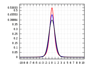
The effects of kurtosis are illustrated using a parametric family of distributions whose kurtosis can be adjusted while their lower-order moments and cumulants remain constant. Consider the Pearson type VII family, which is a special case of the Pearson type IV family restricted to symmetric densities. The probability density function is given by

where a is a scale parameter and m is a shape parameter.
All densities in this family are symmetric. The kth moment exists provided m > (k + 1)/2. For the kurtosis to exist, we require m > 5/2. Then the mean and skewness exist and are both identically zero. Setting a2 = 2m − 3 makes the variance equal to unity. Then the only free parameter is m, which controls the fourth moment (and cumulant) and hence the kurtosis. One can reparameterize with , where is the excess kurtosis as defined above. This yields a one-parameter leptokurtic family with zero mean, unit variance, zero skewness, and arbitrary non-negative excess kurtosis. The reparameterized density is


In the limit as one obtains the density


which is shown as the red curve in the images on the right.
In the other direction as one obtains the standard normal density as the limiting distribution, shown as the black curve.

In the images on the right, the blue curve represents the density with excess kurtosis of 2. The top image shows that leptokurtic densities in this family have a higher peak than the mesokurtic normal density, although this conclusion is only valid for this select family of distributions. The comparatively fatter tails of the leptokurtic densities are illustrated in the second image, which plots the natural logarithm of the Pearson type VII densities: the black curve is the logarithm of the standard normal density, which is a parabola. One can see that the normal density allocates little probability mass to the regions far from the mean ("has thin tails"), compared with the blue curve of the leptokurtic Pearson type VII density with excess kurtosis of 2. Between the blue curve and the black are other Pearson type VII densities with γ2 = 1, 1/2, 1/4, 1/8, and 1/16. The red curve again shows the upper limit of the Pearson type VII family, with (which, strictly speaking, means that the fourth moment does not exist). The red curve decreases the slowest as one moves outward from the origin ("has fat tails").


Other well-known distributions
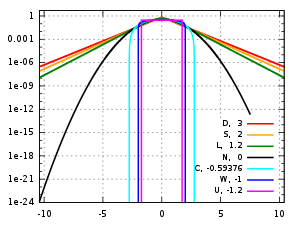
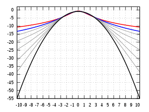
Several well-known, unimodal and symmetric distributions from different parametric families are compared here. Each has a mean and skewness of zero. The parameters have been chosen to result in a variance equal to 1 in each case. The images on the right show curves for the following seven densities, on a linear scale and logarithmic scale:
- D: Laplace distribution, also known as the double exponential distribution, red curve (two straight lines in the log-scale plot), excess kurtosis = 3
- S: hyperbolic secant distribution, orange curve, excess kurtosis = 2
- L: logistic distribution, green curve, excess kurtosis = 1.2
- N: normal distribution, black curve (inverted parabola in the log-scale plot), excess kurtosis = 0
- C: raised cosine distribution, cyan curve, excess kurtosis = −0.593762...
- W: Wigner semicircle distribution, blue curve, excess kurtosis = −1
- U: uniform distribution, magenta curve (shown for clarity as a rectangle in both images), excess kurtosis = −1.2.
Note that in these cases the platykurtic densities have bounded support, whereas the densities with positive or zero excess kurtosis are supported on the whole real line.
One cannot infer that high or low kurtosis distributions have the characteristics indicated by these examples. There exist platykurtic densities with infinite support,
- e.g., exponential power distributions with sufficiently large shape parameter b
and there exist leptokurtic densities with finite support.
- e.g., a distribution that is uniform between −3 and −0.3, between −0.3 and 0.3, and between 0.3 and 3, with the same density in the (−3, −0.3) and (0.3, 3) intervals, but with 20 times more density in the (−0.3, 0.3) interval
Also, there exist platykurtic densities with infinite peakedness,
- e.g., an equal mixture of the beta distribution with parameters 0.5 and 1 with its reflection about 0.0
and there exist leptokurtic densities that appear flat-topped,
- e.g., a mixture of distribution that is uniform between -1 and 1 with a T(4.0000001) Student's t-distribution, with mixing probabilities 0.999 and 0.001.
Sample kurtosis
Definition
For a sample of n values the sample excess kurtosis is

where m4 is the fourth sample moment about the mean, m2 is the second sample moment about the mean (that is, the sample variance), xi is the ith value, and is the sample mean.

This formula has the simpler representation,

where the values are the standardized data values using the standard deviation defined using n rather than n − 1 in the denominator.

For example, suppose the data values are 0, 3, 4, 1, 2, 3, 0, 2, 1, 3, 2, 0, 2, 2, 3, 2, 5, 2, 3, 999.
Then the values are −0.239, −0.225, −0.221, −0.234, −0.230, −0.225, −0.239, −0.230, −0.234, −0.225, −0.230, −0.239, −0.230, −0.230, −0.225, −0.230, −0.216, −0.230, −0.225, 4.359
and the values are 0.003, 0.003, 0.002, 0.003, 0.003, 0.003, 0.003, 0.003, 0.003, 0.003, 0.003, 0.003, 0.003, 0.003, 0.003, 0.003, 0.002, 0.003, 0.003, 360.976.

The average of these values is 18.05 and the excess kurtosis is thus 18.05 − 3 = 15.05. This example makes it clear that data near the "middle" or "peak" of the distribution do not contribute to the kurtosis statistic, hence kurtosis does not measure "peakedness". It is simply a measure of the outlier, 999 in this example.
Upper bound
An upper bound for the sample kurtosis of n (n > 2) real numbers is[13]

where is the sample skewness .


Variance under normality
The variance of the sample kurtosis of a sample of size n from the normal distribution is[14]

Stated differently, under the assumption that the underlying random variable is normally distributed, it can be shown that .[15]:Page number needed


Estimators of population kurtosis
Given a sub-set of samples from a population, the sample excess kurtosis above is a biased estimator of the population excess kurtosis. An alternative estimator of the population excess kurtosis is defined as follows:

where k4 is the unique symmetric unbiased estimator of the fourth cumulant, k2 is the unbiased estimate of the second cumulant (identical to the unbiased estimate of the sample variance), m4 is the fourth sample moment about the mean, m2 is the second sample moment about the mean, xi is the ith value, and is the sample mean. Unfortunately, is itself generally biased. For the normal distribution it is unbiased.[3]


Applications
The sample kurtosis is a useful measure of whether there is a problem with outliers in a data set. Larger kurtosis indicates a more serious outlier problem, and may lead the researcher to choose alternative statistical methods.
D'Agostino's K-squared test is a goodness-of-fit normality test based on a combination of the sample skewness and sample kurtosis, as is the Jarque–Bera test for normality.
For non-normal samples, the variance of the sample variance depends on the kurtosis; for details, please see variance.
Pearson's definition of kurtosis is used as an indicator of intermittency in turbulence.[16]
A concrete example is the following lemma by , He, Zhang and Zhang[17]: Assume a random variable has expectation , variance and kurtosis . Assume we sample many independent copies. Then


- .

This shows that with many samples, we will see one that is above the expectation with probability at least . In other words: If the kurtosis is large, we might see a lot values either all below or above the mean.


Kurtosis convergence
Applying band-pass filters to digital images, kurtosis values tend to be uniform, independent of the range of the filter. This behavior, termed kurtosis convergence, can be used to detect image splicing in forensic analysis.[18]
Other measures
A different measure of "kurtosis" is provided by using L-moments instead of the ordinary moments.[19][20]
See also
| Wikimedia Commons has media related to Kurtosis. |
References
- Pearson, Karl (1905), "Das Fehlergesetz und seine Verallgemeinerungen durch Fechner und Pearson. A Rejoinder" [The Error Law and its Generalizations by Fechner and Pearson. A Rejoinder], Biometrika, 4 (1–2): 169–212, doi:10.1093/biomet/4.1-2.169, JSTOR 2331536
- Westfall, Peter H. (2014), "Kurtosis as Peakedness, 1905 - 2014. R.I.P.", The American Statistician, 68 (3): 191–195, doi:10.1080/00031305.2014.917055, PMC 4321753, PMID 25678714
- Joanes, Derrick N.; Gill, Christine A. (1998), "Comparing measures of sample skewness and kurtosis", Journal of the Royal Statistical Society, Series D, 47 (1): 183–189, doi:10.1111/1467-9884.00122, JSTOR 2988433
- Pearson, Karl (1916), "Mathematical Contributions to the Theory of Evolution. — XIX. Second Supplement to a Memoir on Skew Variation.", Philosophical Transactions of the Royal Society of London A, 216 (546): 429–457, doi:10.1098/rsta.1916.0009, JSTOR 91092
- Balanda, Kevin P.; MacGillivray, Helen L. (1988), "Kurtosis: A Critical Review", The American Statistician, 42 (2): 111–119, doi:10.2307/2684482, JSTOR 2684482
- Darlington, Richard B. (1970), "Is Kurtosis Really 'Peakedness'?", The American Statistician, 24 (2): 19–22, doi:10.1080/00031305.1970.10478885, JSTOR 2681925
- Moors, J. J. A. (1986), "The meaning of kurtosis: Darlington reexamined", The American Statistician, 40 (4): 283–284, doi:10.1080/00031305.1986.10475415, JSTOR 2684603
- "Lepto-".
- Benveniste, Albert; Goursat, Maurice; Ruget, Gabriel (1980), "Robust identification of a nonminimum phase system: Blind adjustment of a linear equalizer in data communications", IEEE Transactions on Automatic Control, 25 (3): 385–399, doi:10.1109/tac.1980.1102343
- http://www.yourdictionary.com/platy-prefix
- Kahane, Jean-Pierre (1960), "Propriétés locales des fonctions à séries de Fourier aléatoires" [Local properties of functions in terms of random Fourier series], Studia Mathematica (in French), 19 (1): 1–25, doi:10.4064/sm-19-1-1-25
- Buldygin, Valerii V.; Kozachenko, Yuriy V. (1980), "Sub-Gaussian random variables", Ukrainian Mathematical Journal, 32 (6): 483–489, doi:10.1007/BF01087176
- Sharma, Rajesh; Bhandari, Rajeev K. (2015), "Skewness, kurtosis and Newton's inequality", Rocky Mountain Journal of Mathematics, 45 (5): 1639–1643, doi:10.1216/RMJ-2015-45-5-1639
- Fisher, Ronald A. (1930), "The Moments of the Distribution for Normal Samples of Measures of Departure from Normality", Proceedings of the Royal Society A, 130 (812): 16–28, doi:10.1098/rspa.1930.0185, JSTOR 95586
- Kendall, Maurice G.; Stuart, Alan, The Advanced Theory of Statistics, Volume 1: Distribution Theory (3rd ed.), London, UK: Charles Griffin & Company Limited, ISBN 0-85264-141-9
- Sandborn, Virgil A. (1959), "Measurements of Intermittency of Turbulent Motion in a Boundary Layer", Journal of Fluid Mechanics, 6 (2): 221–240, doi:10.1017/S0022112059000581
- He, S.; Zhang, J.; Zhang, S. (2010). "Bounding probability of small deviation: A fourth moment approach". Mathematics of Operations Research. 35 (1): 208–232. doi:10.1287/moor.1090.0438.
- Pan, Xunyu; Zhang, Xing; Lyu, Siwei (2012), "Exposing Image Splicing with Inconsistent Local Noise Variances", 2012 IEEE International Conference on Computational Photography (ICCP), 28-29 April 2012; Seattle, WA, USA: IEEE, doi:10.1109/ICCPhot.2012.6215223CS1 maint: location (link)
- Hosking, Jonathan R. M. (1992), "Moments or L moments? An example comparing two measures of distributional shape", The American Statistician, 46 (3): 186–189, doi:10.1080/00031305.1992.10475880, JSTOR 2685210
- Hosking, Jonathan R. M. (2006), "On the characterization of distributions by their L-moments", Journal of Statistical Planning and Inference, 136 (1): 193–198, doi:10.1016/j.jspi.2004.06.004
Further reading
- Kim, Tae-Hwan; White, Halbert (2003). "On More Robust Estimation of Skewness and Kurtosis: Simulation and Application to the S&P500 Index". Finance Research Letters. 1: 56–70. doi:10.1016/S1544-6123(03)00003-5. Alternative source (Comparison of kurtosis estimators)
- Seier, E.; Bonett, D.G. (2003). "Two families of kurtosis measures". Metrika. 58: 59–70. doi:10.1007/s001840200223.
External links
| Wikiversity has learning resources about Kurtosis |
- Hazewinkel, Michiel, ed. (2001) [1994], "Excess coefficient", Encyclopedia of Mathematics, Springer Science+Business Media B.V. / Kluwer Academic Publishers, ISBN 978-1-55608-010-4
- Kurtosis calculator
- Free Online Software (Calculator) computes various types of skewness and kurtosis statistics for any dataset (includes small and large sample tests)..
- Kurtosis on the Earliest known uses of some of the words of mathematics
- Celebrating 100 years of Kurtosis a history of the topic, with different measures of kurtosis.