Gamma function
In mathematics, the gamma function (represented by the capital letter gamma from the Greek alphabet) is one commonly used extension of the factorial function to complex numbers. The gamma function is defined for all complex numbers except the non-positive integers. For any positive integer


Derived by Daniel Bernoulli, for complex numbers with a positive real part the gamma function is defined via a convergent improper integral:

The gamma function then is defined as the analytic continuation of this integral function to a meromorphic function that is holomorphic in the whole complex plane except the non-positive integers, where the function has simple poles.
The gamma function has no zeroes, so the reciprocal gamma function is an entire function. In fact, the gamma function corresponds to the Mellin transform of the negative exponential function:


Other extensions of the factorial function do exist, but the gamma function is the most popular and useful. It is a component in various probability-distribution functions, and as such it is applicable in the fields of probability and statistics, as well as combinatorics.
Motivation

The gamma function can be seen as a solution to the following interpolation problem:
- "Find a smooth curve that connects the points given by at the positive integer values for ."


A plot of the first few factorials makes clear that such a curve can be drawn, but it would be preferable to have a formula that precisely describes the curve, in which the number of operations does not depend on the size of . The simple formula for the factorial, , cannot be used directly for fractional values of since it is only valid when x is a natural number (or positive integer). There are, relatively speaking, no such simple solutions for factorials; no finite combination of sums, products, powers, exponential functions, or logarithms will suffice to express ; but it is possible to find a general formula for factorials using tools such as integrals and limits from calculus. A good solution to this is the gamma function.[1]


There are infinitely many continuous extensions of the factorial to non-integers: infinitely many curves can be drawn through any set of isolated points. The gamma function is the most useful solution in practice, being analytic (except at the non-positive integers), and it can be defined in several equivalent ways. However, it is not the only analytic function which extends the factorial, as adding to it any analytic function which is zero on the positive integers, such as k sin mπx, will give another function with that property.[1]
A more restrictive property than satisfying the above interpolation is to satisfy the recurrence relation defining a translated version of the factorial function,[2][3]


for x equal to any positive real number. But this would allow for multiplication by any periodic analytic function which evaluates to 1 on the positive integers, such as e k sin mπx. One of several ways to finally resolve the ambiguity comes from the Bohr–Mollerup theorem. It states that when the condition that f be logarithmically convex (or "super-convex"[4]) is added, it uniquely determines f for positive, real inputs. From there, the gamma function can be extended to all real and complex values (except the negative integers and zero) by using the unique analytic continuation of f.[5]
Definition
Main definition
The notation is due to Legendre.[1] If the real part of the complex number z is positive (), then the integral


converges absolutely, and is known as the Euler integral of the second kind. (Euler's integral of the first kind is the beta function.[1]) Using integration by parts, one sees that:

Recognizing that as


We can calculate


Given that and


for all positive integers n. This can be seen as an example of proof by induction.
The identity can be used (or, yielding the same result, analytic continuation can be used) to uniquely extend the integral formulation for to a meromorphic function defined for all complex numbers z, except integers less than or equal to zero.[1] It is this extended version that is commonly referred to as the gamma function.[1]

Alternative definitions
Euler's definition as an infinite product
When seeking to approximate for a complex number , it is effective to first compute for some large integer . Use that to approximate a value for , and then use the recursion relation backwards times, to unwind it to an approximation for . Furthermore, this approximation is exact in the limit as goes to infinity.


Specifically, for a fixed integer , it is the case that


If is not an integer then it is not possible to say whether this equation is true because we have not yet (in this section) defined the factorial function for non-integers. However, we do get a unique extension of the factorial function to the non-integers by insisting that this equation continue to hold when the arbitrary integer is replaced by an arbitrary complex number .

Multiplying both sides by gives

This infinite product converges for all complex numbers except the negative integers, which fail because trying to use the recursion relation backwards through the value involves a division by zero.

Similarly for the gamma function, the definition as an infinite product due to Euler is valid for all complex numbers except the non-positive integers:

By this construction, the gamma function is the unique function that simultaneously satisfies , for all complex numbers except the non-positive integers, and for all complex numbers .[1]


Weierstrass's definition
The definition for the gamma function due to Weierstrass is also valid for all complex numbers z except the non-positive integers:

where is the Euler–Mascheroni constant.[1] This is the Hadamard Product of in a rewritten form. Indeed, since is entire of genus 1 with a simple zero at , we have the product representation


where the product is over the zeros of . Since has simple poles at the non-positive integers, it follows has simple zeros at the nonpositive integers, and so the equation above becomes Weierstrass's formula with in place of . The derivation of the constants and is somewhat technical, but can be accomplished by using some identities involving the Riemann zeta function (see this identity, for instance). See also the Weierstrass factorization theorem.


In terms of generalized Laguerre polynomials
A representation of the incomplete gamma function in terms of generalized Laguerre polynomials is

which converges for and .[6]


Properties
General
Other important functional equations for the gamma function are Euler's reflection formula

which implies

and the Legendre duplication formula

Derivation of Euler's reflection formula |
|---|
|
Since the gamma function can be represented as Integrating by parts times yields which is equal to This can be rewritten as Then, using the functional equation of the gamma function, we get It can be proved that Then Euler's reflection formula follows: |


Derivation of the Legendre duplication formula |
|---|
|
The beta function can be represented as Setting yields After the substitution we get The function is even, hence Now assume Then This implies Since the Legendre duplication formula follows: |


The duplication formula is a special case of the multiplication theorem (See[7], Eq. 5.5.6)

A simple but useful property, which can be seen from the limit definition, is:

In particular, with z = a + bi, this product is

If the real part is an integer or a half-integer, this can be finitely expressed in closed form:

Proof of formulas for integer or half-integer real part |
|---|
|
First, consider the reflection formula applied to . Applying the recurrence relation to the second term, we have which with simple rearrangement gives Second, consider the reflection formula applied to . Formulas for other values of for which the real part is integer or half-integer quickly follow by induction using the recurrence relation in the positive and negative directions. |


Perhaps the best-known value of the gamma function at a non-integer argument is

which can be found by setting in the reflection or duplication formulas, by using the relation to the beta function given below with , or simply by making the substitution in the integral definition of the gamma function, resulting in a Gaussian integral. In general, for non-negative integer values of we have:


where denotes the double factorial of n and, when , . See Particular values of the gamma function for calculated values.


It might be tempting to generalize the result that by looking for a formula for other individual values where is rational, especially because according to Gauss's digamma theorem, it is possible to do so for the closely related digamma function at every rational value. However, these numbers are not known to be expressible by themselves in terms of elementary functions. It has been proved that is a transcendental number and algebraically independent of for any integer and each of the fractions .[8] In general, when computing values of the gamma function, we must settle for numerical approximations.


Another useful limit for asymptotic approximations is:

The derivatives of the gamma function are described in terms of the polygamma function. For example:

For a positive integer m the derivative of the gamma function can be calculated as follows (here is the Euler–Mascheroni constant):


For the th derivative of the gamma function is:


(This can be derived by differentiating the integral form of the gamma function with respect to , and using the technique of differentiation under the integral sign.)
Using the identity

where is the Riemann zeta function, and is a partition of given by


we have in particular

Inequalities
When restricted to the positive real numbers, the gamma function is a strictly logarithmically convex function. This property may be stated in any of the following three equivalent ways:
- For any two positive real numbers and , and for any ,


- For any two positive real numbers x and y with y > x,

- For any positive real number ,

The last of these statements is, essentially by definition, the same as the statement that , where is the polygamma function of order 1. To prove the logarithmic convexity of the gamma function, it therefore suffices to observe that has a series representation which, for positive real x, consists of only positive terms.


Logarithmic convexity and Jensen's inequality together imply, for any positive real numbers and ,


There are also bounds on ratios of gamma functions. The best-known is Gautschi's inequality, which says that for any positive real number x and any s ∈ (0, 1),

Stirling's formula


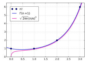
The behavior of for an increasing positive variable is simple. It grows quickly, faster than an exponential function in fact. Asymptotically as , the magnitude of the gamma function is given by Stirling's formula


where the symbol implies asymptotic convergence. In other words, the ratio of the two sides converges to 1 as .[1]


Residues
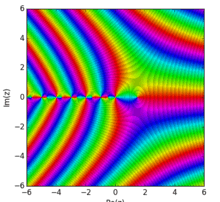
The behavior for non-positive is more intricate. Euler's integral does not converge for , but the function it defines in the positive complex half-plane has a unique analytic continuation to the negative half-plane. One way to find that analytic continuation is to use Euler's integral for positive arguments and extend the domain to negative numbers by repeated application of the recurrence formula,[1]


choosing such that is positive. The product in the denominator is zero when equals any of the integers . Thus, the gamma function must be undefined at those points to avoid division by zero; it is a meromorphic function with simple poles at the non-positive integers.[1]


For a function of a complex variable , at a simple pole , the residue of is given by:


For the simple pole we rewrite recurrence formula as:


The numerator at is

and the denominator

So the residues of the gamma function at those points are:

The gamma function is non-zero everywhere along the real line, although it comes arbitrarily close to zero as z → −∞. There is in fact no complex number for which , and hence the reciprocal gamma function is an entire function, with zeros at .[1]


Minima
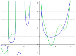
The gamma function has a local minimum at zmin ≈ +1.46163214496836234126 (truncated) where it attains the value Γ(zmin) ≈ +0.88560319441088870027 (truncated). The gamma function must alternate sign between the poles because the product in the forward recurrence contains an odd number of negative factors if the number of poles between and is odd, and an even number if the number of poles is even.[9]
Integral representations
There are many formulas, besides the Euler integral of the second kind, that express the gamma function as an integral. For instance, when the real part of z is positive,[10]

Binet's first integral formula for the gamma function states that, when the real part of z is positive, then:[11]

The integral on the right-hand side may be interpreted as a Laplace transform. That is,

Binet's second integral formula states that, again when the real part of z is positive, then:[12]

Let C be a Hankel contour, meaning a path that begins and ends at the point ∞ on the Riemann sphere, whose unit tangent vector converges to −1 at the start of the path and to 1 at the end, which has winding number 1 around 0, and which does not cross [0, ∞). Fix a branch of by taking a branch cut along [0, ∞) and by taking to be real when t is on the negative real axis. Assume z is not an integer. Then Hankel's formula for the gamma function is:[13]


where is interpreted as . The reflection formula leads to the closely related expression


again valid whenever z is not an integer.
Fourier series expansion
The logarithm of the gamma function has the following Fourier series expansion for


which was for a long time attributed to Ernst Kummer, who derived it in 1847.[14][15] However, Iaroslav Blagouchine discovered that Carl Johan Malmsten first derived this series in 1842.[16][17]
Raabe's formula
In 1840 Joseph Ludwig Raabe proved that

In particular, if then


The latter can be derived taking the logarithm in the above multiplication formula, which gives an expression for the Riemann sum of the integrand. Taking the limit for gives the formula.

Pi function
An alternative notation which was originally introduced by Gauss and which was sometimes used is the -function, which in terms of the gamma function is


so that for every non-negative integer .

Using the pi function the reflection formula takes on the form

where sinc is the normalized sinc function, while the multiplication theorem takes on the form

We also sometimes find

which is an entire function, defined for every complex number, just like the reciprocal gamma function. That is entire entails it has no poles, so , like , has no zeros.


The volume of an n-ellipsoid with radii r1, …, rn can be expressed as

Relation to other functions
- In the first integral above, which defines the gamma function, the limits of integration are fixed. The upper and lower incomplete gamma functions are the functions obtained by allowing the lower or upper (respectively) limit of integration to vary.
- The gamma function is related to the beta function by the formula

- The logarithmic derivative of the gamma function is called the digamma function; higher derivatives are the polygamma functions.
- The analog of the gamma function over a finite field or a finite ring is the Gaussian sums, a type of exponential sum.
- The reciprocal gamma function is an entire function and has been studied as a specific topic.
- The gamma function also shows up in an important relation with the Riemann zeta function, .
- It also appears in the following formula:
- which is valid only for .
- The logarithm of the gamma function satisfies the following formula due to Lerch:
- where is the Hurwitz zeta function, is the Riemann zeta function and the prime (′) denotes differentiation in the first variable.


- The gamma function is related to the stretched exponential function. For instance, the moments of that function are

Particular values
Including up to the first 20 digits after the decimal point, some particular values of the gamma function are:

The complex-valued gamma function is undefined for non-positive integers, but in these cases the value can be defined in the Riemann sphere as ∞. The reciprocal gamma function is well defined and analytic at these values (and in the entire complex plane):

The log-gamma function

Because the gamma and factorial functions grow so rapidly for moderately large arguments, many computing environments include a function that returns the natural logarithm of the gamma function (often given the name lgamma or lngamma in programming environments or gammaln in spreadsheets); this grows much more slowly, and for combinatorial calculations allows adding and subtracting logs instead of multiplying and dividing very large values. It is often defined as[18]

The digamma function, which is the derivative of this function, is also commonly seen. In the context of technical and physical applications, e.g. with wave propagation, the functional equation

is often used since it allows one to determine function values in one strip of width 1 in z from the neighbouring strip. In particular, starting with a good approximation for a z with large real part one may go step by step down to the desired z. Following an indication of Carl Friedrich Gauss, Rocktaeschel (1922) proposed for an approximation for large Re(z):


This can be used to accurately approximate ln(Γ(z)) for z with a smaller Re(z) via (P.E.Böhmer, 1939)

A more accurate approximation can be obtained by using more terms from the asymptotic expansions of ln(Γ(z)) and Γ(z), which are based on Stirling's approximation.
- as |z| → ∞ at constant |arg(z)| < π.

In a more "natural" presentation:
- as |z| → ∞ at constant |arg(z)| < π.

The coefficients of the terms with k > 1 of z−k + 1 in the last expansion are simply

where the Bk are the Bernoulli numbers.
Properties
The Bohr–Mollerup theorem states that among all functions extending the factorial functions to the positive real numbers, only the gamma function is log-convex, that is, its natural logarithm is convex on the positive real axis.
In a certain sense, the ln(Γ) function is the more natural form; it makes some intrinsic attributes of the function clearer. A striking example is the Taylor series of ln(Γ) around 1:

with ζ(k) denoting the Riemann zeta function at k.
So, using the following property:

we can find an integral representation for the ln(Γ) function:

or, setting z = 1 and calculating γ:

There also exist special formulas for the logarithm of the gamma function for rational z. For instance, if and are integers with and , then


see.[19] This formula is sometimes used for numerical computation, since the integrand decreases very quickly.
Integration over log-gamma
The integral

can be expressed in terms of the Barnes G-function[20][21] (see Barnes G-function for a proof):

where Re(z) > −1.
It can also be written in terms of the Hurwitz zeta function:[22][23]

When it follows that


and this is a consequence of Raabe's formula as well. O. Espinosa and V. Moll derived a similar formula for the integral of the square of :[24]


where is .


D. H. Bailey and his co-authors[25] gave an evaluation for

when in terms of the Tornheim-Witten zeta function and its derivatives.

In addition, it is also known that[26]

Approximations
Complex values of the gamma function can be computed numerically with arbitrary precision using Stirling's approximation or the Lanczos approximation.
The gamma function can be computed to fixed precision for by applying integration by parts to Euler's integral. For any positive number x the gamma function can be written


When Re(z) ∈ [1,2] and , the absolute value of the last integral is smaller than . By choosing a large enough , this last expression can be made smaller than for any desired value . Thus, the gamma function can be evaluated to bits of precision with the above series.


A fast algorithm for calculation of the Euler gamma function for any algebraic argument (including rational) was constructed by E.A. Karatsuba,[27][28][29]
For arguments that are integer multiples of 1/24, the gamma function can also be evaluated quickly using arithmetic–geometric mean iterations (see particular values of the gamma function and Borwein & Zucker (1992)).
Applications
One author describes the gamma function as "Arguably, the most common special function, or the least 'special' of them. The other transcendental functions […] are called 'special' because you could conceivably avoid some of them by staying away from many specialized mathematical topics. On the other hand, the gamma function y = Γ(x) is most difficult to avoid."[30]
Integration problems
The gamma function finds application in such diverse areas as quantum physics, astrophysics and fluid dynamics.[31] The gamma distribution, which is formulated in terms of the gamma function, is used in statistics to model a wide range of processes; for example, the time between occurrences of earthquakes.[32]
The primary reason for the gamma function's usefulness in such contexts is the prevalence of expressions of the type which describe processes that decay exponentially in time or space. Integrals of such expressions can occasionally be solved in terms of the gamma function when no elementary solution exists. For example, if f is a power function and g is a linear function, a simple change of variables gives the evaluation


The fact that the integration is performed along the entire positive real line might signify that the gamma function describes the cumulation of a time-dependent process that continues indefinitely, or the value might be the total of a distribution in an infinite space.
It is of course frequently useful to take limits of integration other than 0 and ∞ to describe the cumulation of a finite process, in which case the ordinary gamma function is no longer a solution; the solution is then called an incomplete gamma function. (The ordinary gamma function, obtained by integrating across the entire positive real line, is sometimes called the complete gamma function for contrast.)
An important category of exponentially decaying functions is that of Gaussian functions

and integrals thereof, such as the error function. There are many interrelations between these functions and the gamma function; notably, the factor obtained by evaluating is the "same" as that found in the normalizing factor of the error function and the normal distribution.


The integrals we have discussed so far involve transcendental functions, but the gamma function also arises from integrals of purely algebraic functions. In particular, the arc lengths of ellipses and of the lemniscate, which are curves defined by algebraic equations, are given by elliptic integrals that in special cases can be evaluated in terms of the gamma function. The gamma function can also be used to calculate "volume" and "area" of n-dimensional hyperspheres.
Calculating products
The gamma function's ability to generalize factorial products immediately leads to applications in many areas of mathematics; in combinatorics, and by extension in areas such as probability theory and the calculation of power series. Many expressions involving products of successive integers can be written as some combination of factorials, the most important example perhaps being that of the binomial coefficient

The example of binomial coefficients motivates why the properties of the gamma function when extended to negative numbers are natural. A binomial coefficient gives the number of ways to choose k elements from a set of n elements; if k > n, there are of course no ways. If k > n, (n − k)! is the factorial of a negative integer and hence infinite if we use the gamma function definition of factorials—dividing by infinity gives the expected value of 0.
We can replace the factorial by a gamma function to extend any such formula to the complex numbers. Generally, this works for any product wherein each factor is a rational function of the index variable, by factoring the rational function into linear expressions. If P and Q are monic polynomials of degree m and n with respective roots p1, …, pm and q1, …, qn, we have

If we have a way to calculate the gamma function numerically, it is a breeze to calculate numerical values of such products. The number of gamma functions in the right-hand side depends only on the degree of the polynomials, so it does not matter whether b − a equals 5 or 105. By taking the appropriate limits, the equation can also be made to hold even when the left-hand product contains zeros or poles.
By taking limits, certain rational products with infinitely many factors can be evaluated in terms of the gamma function as well. Due to the Weierstrass factorization theorem, analytic functions can be written as infinite products, and these can sometimes be represented as finite products or quotients of the gamma function. We have already seen one striking example: the reflection formula essentially represents the sine function as the product of two gamma functions. Starting from this formula, the exponential function as well as all the trigonometric and hyperbolic functions can be expressed in terms of the gamma function.
More functions yet, including the hypergeometric function and special cases thereof, can be represented by means of complex contour integrals of products and quotients of the gamma function, called Mellin–Barnes integrals.
Analytic number theory
An elegant and deep application of the gamma function is in the study of the Riemann zeta function. A fundamental property of the Riemann zeta function is its functional equation:

Among other things, this provides an explicit form for the analytic continuation of the zeta function to a meromorphic function in the complex plane and leads to an immediate proof that the zeta function has infinitely many so-called "trivial" zeros on the real line. Borwein et al. call this formula "one of the most beautiful findings in mathematics".[33] Another champion for that title might be

Both formulas were derived by Bernhard Riemann in his seminal 1859 paper "Über die Anzahl der Primzahlen unter einer gegebenen Größe" ("On the Number of Prime Numbers less than a Given Quantity"), one of the milestones in the development of analytic number theory—the branch of mathematics that studies prime numbers using the tools of mathematical analysis. Factorial numbers, considered as discrete objects, are an important concept in classical number theory because they contain many prime factors, but Riemann found a use for their continuous extension that arguably turned out to be even more important.
History
The gamma function has caught the interest of some of the most prominent mathematicians of all time. Its history, notably documented by Philip J. Davis in an article that won him the 1963 Chauvenet Prize, reflects many of the major developments within mathematics since the 18th century. In the words of Davis, "each generation has found something of interest to say about the gamma function. Perhaps the next generation will also."[1]
18th century: Euler and Stirling

The problem of extending the factorial to non-integer arguments was apparently first considered by Daniel Bernoulli and Christian Goldbach in the 1720s, and was solved at the end of the same decade by Leonhard Euler. Euler gave two different definitions: the first was not his integral but an infinite product,

of which he informed Goldbach in a letter dated October 13, 1729. He wrote to Goldbach again on January 8, 1730, to announce his discovery of the integral representation

which is valid for n > 0. By the change of variables t = −ln s, this becomes the familiar Euler integral. Euler published his results in the paper "De progressionibus transcendentibus seu quarum termini generales algebraice dari nequeunt" ("On transcendental progressions, that is, those whose general terms cannot be given algebraically"), submitted to the St. Petersburg Academy on November 28, 1729.[34] Euler further discovered some of the gamma function's important functional properties, including the reflection formula.
James Stirling, a contemporary of Euler, also attempted to find a continuous expression for the factorial and came up with what is now known as Stirling's formula. Although Stirling's formula gives a good estimate of n!, also for non-integers, it does not provide the exact value. Extensions of his formula that correct the error were given by Stirling himself and by Jacques Philippe Marie Binet.
19th century: Gauss, Weierstrass and Legendre

Carl Friedrich Gauss rewrote Euler's product as

and used this formula to discover new properties of the gamma function. Although Euler was a pioneer in the theory of complex variables, he does not appear to have considered the factorial of a complex number, as instead Gauss first did.[35] Gauss also proved the multiplication theorem of the gamma function and investigated the connection between the gamma function and elliptic integrals.
Karl Weierstrass further established the role of the gamma function in complex analysis, starting from yet another product representation,

where γ is the Euler–Mascheroni constant. Weierstrass originally wrote his product as one for 1/Γ, in which case it is taken over the function's zeros rather than its poles. Inspired by this result, he proved what is known as the Weierstrass factorization theorem—that any entire function can be written as a product over its zeros in the complex plane; a generalization of the fundamental theorem of algebra.
The name gamma function and the symbol Γ were introduced by Adrien-Marie Legendre around 1811; Legendre also rewrote Euler's integral definition in its modern form. Although the symbol is an upper-case Greek gamma, there is no accepted standard for whether the function name should be written "gamma function" or "Gamma function" (some authors simply write "Γ-function"). The alternative "pi function" notation Π(z) = z! due to Gauss is sometimes encountered in older literature, but Legendre's notation is dominant in modern works.
It is justified to ask why we distinguish between the "ordinary factorial" and the gamma function by using distinct symbols, and particularly why the gamma function should be normalized to Γ(n + 1) = n! instead of simply using "Γ(n) = n!". Consider that the notation for exponents, xn, has been generalized from integers to complex numbers xz without any change. Legendre's motivation for the normalization does not appear to be known, and has been criticized as cumbersome by some (the 20th-century mathematician Cornelius Lanczos, for example, called it "void of any rationality" and would instead use z!).[36] Legendre's normalization does simplify a few formulae, but complicates most others. From a modern point of view, the Legendre normalization of the Gamma function is the integral of the additive character e−x against the multiplicative character xz with respect to the Haar measure on the Lie group R+. Thus this normalization makes it clearer that the gamma function is a continuous analogue of a Gauss sum.

19th–20th centuries: characterizing the gamma function
It is somewhat problematic that a large number of definitions have been given for the gamma function. Although they describe the same function, it is not entirely straightforward to prove the equivalence. Stirling never proved that his extended formula corresponds exactly to Euler's gamma function; a proof was first given by Charles Hermite in 1900.[37] Instead of finding a specialized proof for each formula, it would be desirable to have a general method of identifying the gamma function.
One way to prove would be to find a differential equation that characterizes the gamma function. Most special functions in applied mathematics arise as solutions to differential equations, whose solutions are unique. However, the gamma function does not appear to satisfy any simple differential equation. Otto Hölder proved in 1887 that the gamma function at least does not satisfy any algebraic differential equation by showing that a solution to such an equation could not satisfy the gamma function's recurrence formula, making it a transcendentally transcendental function. This result is known as Hölder's theorem.
A definite and generally applicable characterization of the gamma function was not given until 1922. Harald Bohr and Johannes Mollerup then proved what is known as the Bohr–Mollerup theorem: that the gamma function is the unique solution to the factorial recurrence relation that is positive and logarithmically convex for positive z and whose value at 1 is 1 (a function is logarithmically convex if its logarithm is convex).
The Bohr–Mollerup theorem is useful because it is relatively easy to prove logarithmic convexity for any of the different formulas used to define the gamma function. Taking things further, instead of defining the gamma function by any particular formula, we can choose the conditions of the Bohr–Mollerup theorem as the definition, and then pick any formula we like that satisfies the conditions as a starting point for studying the gamma function. This approach was used by the Bourbaki group.
Borwein & Corless[38] review three centuries of work on the gamma function.
Reference tables and software
Although the gamma function can be calculated virtually as easily as any mathematically simpler function with a modern computer—even with a programmable pocket calculator—this was of course not always the case. Until the mid-20th century, mathematicians relied on hand-made tables; in the case of the gamma function, notably a table computed by Gauss in 1813 and one computed by Legendre in 1825.

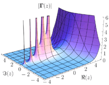
Tables of complex values of the gamma function, as well as hand-drawn graphs, were given in Tables of Higher Functions by Jahnke and Emde, first published in Germany in 1909. According to Michael Berry, "the publication in J&E of a three-dimensional graph showing the poles of the gamma function in the complex plane acquired an almost iconic status."[39]
There was in fact little practical need for anything but real values of the gamma function until the 1930s, when applications for the complex gamma function were discovered in theoretical physics. As electronic computers became available for the production of tables in the 1950s, several extensive tables for the complex gamma function were published to meet the demand, including a table accurate to 12 decimal places from the U.S. National Bureau of Standards.[1]
Abramowitz and Stegun became the standard reference for this and many other special functions after its publication in 1964.
Double-precision floating-point implementations of the gamma function and its logarithm are now available in most scientific computing software and special functions libraries, for example TK Solver, Matlab, GNU Octave, and the GNU Scientific Library. The gamma function was also added to the C standard library (math.h). Arbitrary-precision implementations are available in most computer algebra systems, such as Mathematica and Maple. PARI/GP, MPFR and MPFUN contain free arbitrary-precision implementations. A little-known feature of the calculator app included with the Android operating system is that it will accept fractional values as input to the factorial function and return the equivalent gamma function value. The same is true for Windows Calculator (in scientific mode).
See also
Notes
- Davis, P. J. (1959). "Leonhard Euler's Integral: A Historical Profile of the Gamma Function". American Mathematical Monthly. 66 (10): 849–869. doi:10.2307/2309786. JSTOR 2309786. Retrieved 3 December 2016.
- Beals, Richard; Wong, Roderick (2010). Special Functions: A Graduate Text. Cambridge University Press. p. 28. ISBN 978-1-139-49043-6. Extract of page 28
- Ross, Clay C. (2013). Differential Equations: An Introduction with Mathematica (illustrated ed.). Springer Science & Business Media. p. 293. ISBN 978-1-4757-3949-7. Expression G.2 on page 293
- Kingman, J. F. C. (1961). "A Convexity Property of Positive Matrices". The Quarterly Journal of Mathematics. 12 (1): 283–284. Bibcode:1961QJMat..12..283K. doi:10.1093/qmath/12.1.283.
- Weisstein, Eric W. "Bohr–Mollerup Theorem". MathWorld.
- Askey, R. A.; Roy, R. (2010), "Series Expansions", in Olver, Frank W. J.; Lozier, Daniel M.; Boisvert, Ronald F.; Clark, Charles W. (eds.), NIST Handbook of Mathematical Functions, Cambridge University Press, ISBN 978-0-521-19225-5, MR 2723248
- Askey, R. A.; Roy, R. (2010), "Series Expansions", in Olver, Frank W. J.; Lozier, Daniel M.; Boisvert, Ronald F.; Clark, Charles W. (eds.), NIST Handbook of Mathematical Functions, Cambridge University Press, ISBN 978-0-521-19225-5, MR 2723248
- Waldschmidt, M. (2006). "Transcendence of Periods: The State of the Art" (PDF). Pure Appl. Math. Quart. 2 (2): 435–463. doi:10.4310/pamq.2006.v2.n2.a3.
- Weisstein, Eric W. "Gamma Function". MathWorld.
- Whittaker and Watson, 12.2 example 1.
- Whittaker and Watson, 12.31.
- Whittaker and Watson, 12.32.
- Whittaker and Watson, 12.22.
- Bateman, Harry; Erdélyi, Arthur (1955). Higher Transcendental Functions. McGraw-Hill.
- Srivastava, H. M.; Choi, J. (2001). Series Associated with the Zeta and Related Functions. The Netherlands: Kluwer Academic.
- Blagouchine, Iaroslav V. (2014). "Rediscovery of Malmsten's integrals, their evaluation by contour integration methods and some related results". Ramanujan J. 35 (1): 21–110. doi:10.1007/s11139-013-9528-5.
- Blagouchine, Iaroslav V. (2016). "Erratum and Addendum to "Rediscovery of Malmsten's integrals, their evaluation by contour integration methods and some related results"". Ramanujan J. 42 (3): 777–781. doi:10.1007/s11139-015-9763-z.
- "Log Gamma Function". Wolfram MathWorld. Retrieved 3 January 2019.
- Blagouchine, Iaroslav V. (2015). "A theorem for the closed-form evaluation of the first generalized Stieltjes constant at rational arguments and some related summations". Journal of Number Theory. 148: 537–592. arXiv:1401.3724. doi:10.1016/j.jnt.2014.08.009.
- Alexejewsky, W. P. (1894). "Über eine Classe von Funktionen, die der Gammafunktion analog sind" [On a class of functions analogous to the gamma function]. Leipzig Weidmanncshe Buchhandluns. 46: 268–275.
- Barnes, E. W. (1899). "The theory of the G-function". Quart. J. Math. 31: 264–314.
- Adamchik, Victor S. (1998). "Polygamma functions of negative order". J. Comput. Appl. Math. 100 (2): 191–199. doi:10.1016/S0377-0427(98)00192-7.
- Gosper, R. W. (1997). " in special functions, q-series and related topics". J. Am. Math. Soc. 14.
- Espinosa, Olivier; Moll, Victor H. (2002). "On Some Integrals Involving the Hurwitz Zeta Function: Part 1". The Ramanujan Journal. 6: 159–188. doi:10.1023/A:1015706300169.
- Bailey, David H.; Borwein, David; Borwein, Jonathan M. (2015). "On Eulerian log-gamma integrals and Tornheim-Witten zeta functions". The Ramanujan Journal. 36: 43–68. doi:10.1007/s11139-012-9427-1.
- Amdeberhan, T.; Coffey, Mark W.; Espinosa, Olivier; Koutschan, Christoph; Manna, Dante V.; Moll, Victor H. (2011). "Integrals of powers of loggamma". Proc. Amer. Math. Soc. 139 (2): 535–545. doi:10.1090/S0002-9939-2010-10589-0.
- E.A. Karatsuba, Fast evaluation of transcendental functions. Probl. Inf. Transm. Vol.27, No.4, pp. 339–360 (1991).
- E.A. Karatsuba, On a new method for fast evaluation of transcendental functions. Russ. Math. Surv. Vol.46, No.2, pp. 246–247 (1991).
- E.A. Karatsuba "Fast Algorithms and the FEE Method".
- Michon, G. P. "Trigonometry and Basic Functions Archived 9 January 2010 at the Wayback Machine". Numericana. Retrieved May 5, 2007.
- Chaudry, M. A. & Zubair, S. M. (2001). On A Class of Incomplete Gamma Functions with Applications. p. 37
- Rice, J. A. (1995). Mathematical Statistics and Data Analysis (Second Edition). p. 52–53
- Borwein, J., Bailey, D. H. & Girgensohn, R. (2003). Experimentation in Mathematics. A. K. Peters. p. 133. ISBN 978-1-56881-136-9.CS1 maint: multiple names: authors list (link)
- Euler's paper was published in Commentarii academiae scientiarum Petropolitanae 5, 1738, 36–57. See E19 -- De progressionibus transcendentibus seu quarum termini generales algebraice dari nequeunt, from The Euler Archive, which includes a scanned copy of the original article.
- Remmert, R. (2006). Classical Topics in Complex Function Theory. Translated by Kay, L. D. Springer. ISBN 978-0-387-98221-2.
- Lanczos, C. (1964). "A precision approximation of the gamma function". J. SIAM Numer. Anal. Ser. B. 1.
- Knuth, D. E. (1997). The Art of Computer Programming, Volume 1 (Fundamental Algorithms). Addison-Wesley.
- Borwein, Jonathan M.; Corless, Robert M. (2017). "Gamma and Factorial in the Monthly". American Mathematical Monthly. Mathematical Association of America. 125 (5): 400–24. arXiv:1703.05349. Bibcode:2017arXiv170305349B. doi:10.1080/00029890.2018.1420983.
- Berry, M. (April 2001). "Why are special functions special?". Physics Today.

- This article incorporates material from the Citizendium article "Gamma function", which is licensed under the Creative Commons Attribution-ShareAlike 3.0 Unported License but not under the GFDL.
Further reading
- Abramowitz, Milton; Stegun, Irene A., eds. (1972). "Chapter 6". Handbook of Mathematical Functions with Formulas, Graphs, and Mathematical Tables. New York: Dover.
- Andrews, G. E.; Askey, R.; Roy, R. (1999). "Chapter 1 (Gamma and Beta functions)". Special Functions. New York: Cambridge University Press. ISBN 978-0-521-78988-2.
- Artin, Emil (2006). "The Gamma Function". In Rosen, Michael (ed.). Exposition by Emil Artin: a selection. History of Mathematics. 30. Providence, RI: American Mathematical Society.
- Askey, R.; Roy, R. (2010), "Gamma function", in Olver, Frank W. J.; Lozier, Daniel M.; Boisvert, Ronald F.; Clark, Charles W. (eds.), NIST Handbook of Mathematical Functions, Cambridge University Press, ISBN 978-0-521-19225-5, MR 2723248
- Birkhoff, George D. (1913). "Note on the gamma function". Bull. Amer. Math. Soc. 20 (1): 1–10. doi:10.1090/s0002-9904-1913-02429-7. MR 1559418.
- Böhmer, P. E. (1939). Differenzengleichungen und bestimmte Integrale [Differential Equations and Definite Integrals]. Leipzig: Köhler Verlag.
- Davis, Philip J. (1959). "Leonhard Euler's Integral: A Historical Profile of the Gamma Function". American Mathematical Monthly. 66 (10): 849–869. doi:10.2307/2309786. JSTOR 2309786.
- Press, W. H.; Teukolsky, S. A.; Vetterling, W. T.; Flannery, B. P. (2007). "Section 6.1. Gamma Function". Numerical Recipes: The Art of Scientific Computing (3rd ed.). New York: Cambridge University Press. ISBN 978-0-521-88068-8.
- Rocktäschel, O. R. (1922). Methoden zur Berechnung der Gammafunktion für komplexes Argument [Methods for Calculating the Gamma Function for Complex Arguments]. Dresden: Technical University of Dresden.
- Temme, Nico M. (1996). Special Functions: An Introduction to the Classical Functions of Mathematical Physics. New York: John Wiley & Sons. ISBN 978-0-471-11313-3.
- Whittaker, E. T.; Watson, G. N. (1927). A Course of Modern Analysis. Cambridge University Press. ISBN 978-0-521-58807-2.
External links
| Wikimedia Commons has media related to Gamma and related functions. |
- NIST Digital Library of Mathematical Functions:Gamma function
- Pascal Sebah and Xavier Gourdon. Introduction to the Gamma Function. In PostScript and HTML formats.
- C++ reference for
std::tgamma - Examples of problems involving the gamma function can be found at Exampleproblems.com.
- Hazewinkel, Michiel, ed. (2001) [1994], "Gamma function", Encyclopedia of Mathematics, Springer Science+Business Media B.V. / Kluwer Academic Publishers, ISBN 978-1-55608-010-4
- Wolfram gamma function evaluator (arbitrary precision)
- "Gamma". Wolfram Functions Site.
- Volume of n-Spheres and the Gamma Function at MathPages