Geometric mean

In mathematics, the geometric mean is a mean or average, which indicates the central tendency or typical value of a set of numbers by using the product of their values (as opposed to the arithmetic mean which uses their sum). The geometric mean is defined as the $n$ th root of the product of $n$ numbers, i.e., for a set of numbers $x 1, x 2, ..., x n$ , the geometric mean is defined as

\left(\prod _{i=1}^{n}x_{i}\right)^{\frac {1}{n}}={\sqrt[{n}]{x_{1}x_{2}\cdots x_{n}}}

Construction of the geometric mean:

l_{g}

(red) is the geometric mean of

l_{1}

and

l_{2}

,[1][2] in an example in which the line segment

l_{2}\;({\overline {BC}})

is given as a perpendicular to

{\overline {AB}}

, animation at the end 10 s pause.

For instance, the geometric mean of two numbers, say 2 and 8, is just the square root of their product, that is, ${\sqrt {2\cdot 8}}=4$ . As another example, the geometric mean of the three numbers 4, 1, and 1/32 is the cube root of their product (1/8), which is 1/2, that is, ${\sqrt[{3}]{4\cdot 1\cdot 1/32}}=1/2$ .

A geometric mean is often used when comparing different items—finding a single "figure of merit" for these items—when each item has multiple properties that have different numeric ranges.[3] For example, the geometric mean can give a meaningful value to compare two companies which are each rated at 0 to 5 for their environmental sustainability, and are rated at 0 to 100 for their financial viability. If an arithmetic mean were used instead of a geometric mean, the financial viability would have greater weight because its numeric range is larger. That is, a small percentage change in the financial rating (e.g. going from 80 to 90) makes a much larger difference in the arithmetic mean than a large percentage change in environmental sustainability (e.g. going from 2 to 5). The use of a geometric mean normalizes the differently-ranged values, meaning a given percentage change in any of the properties has the same effect on the geometric mean. So, a 20% change in environmental sustainability from 4 to 4.8 has the same effect on the geometric mean as a 20% change in financial viability from 60 to 72.

The geometric mean can be understood in terms of geometry. The geometric mean of two numbers, $a$ and $b$ , is the length of one side of a square whose area is equal to the area of a rectangle with sides of lengths $a$ and $b$ . Similarly, the geometric mean of three numbers, $a$ , $b$ , and $c$ , is the length of one edge of a cube whose volume is the same as that of a cuboid with sides whose lengths are equal to the three given numbers.

The geometric mean applies only to positive numbers.[4] It is also often used for a set of numbers whose values are meant to be multiplied together or are exponential in nature, such as data on the growth of the human population or interest rates of a financial investment.

The geometric mean is also one of the three classical Pythagorean means, together with the aforementioned arithmetic mean and the harmonic mean. For all positive data sets containing at least one pair of unequal values, the harmonic mean is always the least of the three means, while the arithmetic mean is always the greatest of the three and the geometric mean is always in between (see Inequality of arithmetic and geometric means.)

Calculation

The geometric mean of a data set ${\textstyle \left\{a_{1},a_{2},\,\ldots ,\,a_{n}\right\}}$ is given by:

\left(\prod _{i=1}^{n}a_{i}\right)^{\frac {1}{n}}={\sqrt[{n}]{a_{1}a_{2}\cdots a_{n}}}.

The above figure uses capital pi notation to show a series of multiplications. Each side of the equal sign shows that a set of values is multiplied in succession (the number of values is represented by "n") to give a total product of the set, and then the nth root of the total product is taken to give the geometric mean of the original set. For example, in a set of four numbers ${\textstyle \{1,2,3,4\}}$ , the product of ${\textstyle 1\times 2\times 3\times 4}$ is ${\textstyle 24}$ , and the geometric mean is the fourth root of 24, or ~ 2.213. The exponent ${\textstyle {\frac {1}{n}}}$ on the left side is equivalent to the taking nth root. For example, ${\textstyle 24^{\frac {1}{4}}={\sqrt[{4}]{24}}}$ .

The geometric mean of a data set is less than the data set's arithmetic mean unless all members of the data set are equal, in which case the geometric and arithmetic means are equal. This allows the definition of the arithmetic-geometric mean, an intersection of the two which always lies in between.

The geometric mean is also the arithmetic-harmonic mean in the sense that if two sequences ( ${\textstyle a_{n}}$ ) and ( ${\textstyle h_{n}}$ ) are defined:

a_{n+1}={\frac {a_{n}+h_{n}}{2}},\quad a_{0}=x

and

h_{n+1}={\frac {2}{{\frac {1}{a_{n}}}+{\frac {1}{h_{n}}}}},\quad h_{0}=y

where ${\textstyle h_{n+1}}$ is the harmonic mean of the previous values of the two sequences, then ${\textstyle a_{n}}$ and ${\textstyle h_{n}}$ will converge to the geometric mean of ${\textstyle x}$ and ${\textstyle y}$ .

This can be seen easily from the fact that the sequences do converge to a common limit (which can be shown by Bolzano–Weierstrass theorem) and the fact that geometric mean is preserved:

{\sqrt {a_{i}h_{i}}}={\sqrt {\frac {a_{i}+h_{i}}{\frac {a_{i}+h_{i}}{h_{i}a_{i}}}}}={\sqrt {\frac {a_{i}+h_{i}}{{\frac {1}{a_{i}}}+{\frac {1}{h_{i}}}}}}={\sqrt {a_{i+1}h_{i+1}}}

Replacing the arithmetic and harmonic mean by a pair of generalized means of opposite, finite exponents yields the same result.

Relationship with logarithms

The geometric mean can also be expressed as the exponential of the arithmetic mean of logarithms.[5] By using logarithmic identities to transform the formula, the multiplications can be expressed as a sum and the power as a multiplication:

When $a_{1},a_{2},\dots ,a_{n}>0$

\left(\prod _{i=1}^{n}a_{i}\right)^{\frac {1}{n}}=\exp \left[{\frac {1}{n}}\sum _{i=1}^{n}\ln a_{i}\right];

additionally, if negative values of the $a_{i}$ are allowed,

\left(\prod _{i=1}^{n}a_{i}\right)^{\frac {1}{n}}=\left(\left(-1\right)^{m}\right)^{\frac {1}{n}}\exp \left[{\frac {1}{n}}\sum _{i=1}^{n}\ln \left|a_{i}\right|\right],

where $m$ is the number of negative numbers.

This is sometimes called the log-average (not to be confused with the logarithmic average). It is simply computing the arithmetic mean of the logarithm-transformed values of $a_{i}$ (i.e., the arithmetic mean on the log scale) and then using the exponentiation to return the computation to the original scale, i.e., it is the generalised f-mean with $f(x)=\log x$ . For example, the geometric mean of 2 and 8 can be calculated as the following, where $b$ is any base of a logarithm (commonly 2, $e$ or 10):

b^{{\frac {1}{2}}\left[\log _{b}(2)+\log _{b}(8)\right]}=4

Related to the above, it can be seen that for a given sample of points $a_{1},\ldots ,a_{n}$ , the geometric mean is the minimizer of $f(a)=\sum _{i=1}^{n}(\log(a_{i})-\log(a))^{2}$ , whereas the arithmetic mean is the minimizer of $f(a)=\sum _{i=1}^{n}(a_{i}-a)^{2}$ . Thus, the geometric mean provides a summary of the samples whose exponent best matches the exponents of the samples (in the least squares sense).

The log form of the geometric mean is generally the preferred alternative for implementation in computer languages because calculating the product of many numbers can lead to an arithmetic overflow or arithmetic underflow. This is less likely to occur with the sum of the logarithms for each number.

Comparison to arithmetic mean

The geometric mean of a non-empty data set of (positive) numbers is always at most their arithmetic mean. Equality is only obtained when all numbers in the data set are equal; otherwise, the geometric mean is smaller. For example, the geometric mean of 242 and 288 equals 264, while their arithmetic mean is 265. In particular, this means that when a set of non-identical numbers is subjected to a mean-preserving spread — that is, the elements of the set are "spread apart" more from each other while leaving the arithmetic mean unchanged — their geometric mean decreases.[6]

Average growth rate

In many cases the geometric mean is the best measure to determine the average growth rate of some quantity. (For example, if in one year sales increases by 80% and the next year by 25%, the end result is the same as that of a constant growth rate of 50%, since the geometric mean of 1.80 and 1.25 is 1.50.) In order to determine the average growth rate, it is not necessary to take the product of the measured growth rates at every step. Let the quantity be given as the sequence $a_{0},a_{1},...,a_{n}$ , where $n$ is the number of steps from the initial to final state. The growth rate between successive measurements $a_{k}$ and $a_{k+1}$ is $a_{k+1}/a_{k}$ . The geometric mean of these growth rates is then just:

\left({\frac {a_{1}}{a_{0}}}{\frac {a_{2}}{a_{1}}}\cdots {\frac {a_{n}}{a_{n-1}}}\right)^{\frac {1}{n}}=\left({\frac {a_{n}}{a_{0}}}\right)^{\frac {1}{n}}.

Application to normalized values

The fundamental property of the geometric mean, which does not hold for any other mean, is that for two sequences $X$ and $Y$ of equal length,

\operatorname {GM} \left({\frac {X_{i}}{Y_{i}}}\right)={\frac {\operatorname {GM} (X_{i})}{\operatorname {GM} (Y_{i})}}

This makes the geometric mean the only correct mean when averaging normalized results; that is, results that are presented as ratios to reference values.[7] This is the case when presenting computer performance with respect to a reference computer, or when computing a single average index from several heterogeneous sources (for example, life expectancy, education years, and infant mortality). In this scenario, using the arithmetic or harmonic mean would change the ranking of the results depending on what is used as a reference. For example, take the following comparison of execution time of computer programs:

	Computer A	Computer B	Computer C
Program 1	1	10	20
Program 2	1000	100	20
Arithmetic mean	500.5	55	20
Geometric mean	31.622 . . .	31.622 . . .	20
Harmonic mean	1.998 . . .	18.182 . . .	20

The arithmetic and geometric means "agree" that computer C is the fastest. However, by presenting appropriately normalized values and using the arithmetic mean, we can show either of the other two computers to be the fastest. Normalizing by A's result gives A as the fastest computer according to the arithmetic mean:

	Computer A	Computer B	Computer C
Program 1	1	10	20
Program 2	1	0.1	0.02
Arithmetic mean	1	5.05	10.01
Geometric mean	1	1	0.632 . . .
Harmonic mean	1	0.198 . . .	0.039 . . .

while normalizing by B's result gives B as the fastest computer according to the arithmetic mean but A as the fastest according to the harmonic mean:

	Computer A	Computer B	Computer C
Program 1	0.1	1	2
Program 2	10	1	0.2
Arithmetic mean	5.05	1	1.1
Geometric mean	1	1	0.632
Harmonic mean	0.198 . . .	1	0.363 . . .

and normalizing by C's result gives C as the fastest computer according to the arithmetic mean but A as the fastest according to the harmonic mean:

	Computer A	Computer B	Computer C
Program 1	0.05	0.5	1
Program 2	50	5	1
Arithmetic mean	25.025	2.75	1
Geometric mean	1.581 . . .	1.581 . . .	1
Harmonic mean	0.099 . . .	0.909 . . .	1

In all cases, the ranking given by the geometric mean stays the same as the one obtained with unnormalized values.

However, this reasoning has been questioned.[8] Giving consistent results is not always equal to giving the correct results. In general, it is more rigorous to assign weights to each of the programs, calculate the average weighted execution time (using the arithmetic mean), and then normalize that result to one of the computers. The three tables above just give a different weight to each of the programs, explaining the inconsistent results of the arithmetic and harmonic means (the first table gives equal weight to both programs, the second gives a weight of 1/1000 to the second program, and the third gives a weight of 1/100 to the second program and 1/10 to the first one). The use of the geometric mean for aggregating performance numbers should be avoided if possible, because multiplying execution times has no physical meaning, in contrast to adding times as in the arithmetic mean. Metrics that are inversely proportional to time (speedup, IPC) should be averaged using the harmonic mean.

The geometric mean can be derived from the generalized mean as its limit as $p$ goes to zero. Similarly, this is possible for the weighted geometric mean.

Applications

Proportional growth

The geometric mean is more appropriate than the arithmetic mean for describing proportional growth, both exponential growth (constant proportional growth) and varying growth; in business the geometric mean of growth rates is known as the compound annual growth rate (CAGR). The geometric mean of growth over periods yields the equivalent constant growth rate that would yield the same final amount.

Suppose an orange tree yields 100 oranges one year and then 180, 210 and 300 the following years, so the growth is 80%, 16.6666% and 42.8571% for each year respectively. Using the arithmetic mean calculates a (linear) average growth of 46.5079% (80% + 16.6666% + 42.8571%, that sum then divided by 3). However, if we start with 100 oranges and let it grow 46.5079% each year, the result is 314 oranges, not 300, so the linear average over-states the year-on-year growth.

Instead, we can use the geometric mean. Growing with 80% corresponds to multiplying with 1.80, so we take the geometric mean of 1.80, 1.166666 and 1.428571, i.e. ${\sqrt[{3}]{1.80\times 1.166666\times 1.428571}}\approx 1.442249$ ; thus the "average" growth per year is 44.2249%. If we start with 100 oranges and let the number grow with 44.2249% each year, the result is 300 oranges.

Financial

The geometric mean has from time to time been used to calculate financial indices (the averaging is over the components of the index). For example, in the past the FT 30 index used a geometric mean.[9] It is also used in the recently introduced "RPIJ" measure of inflation in the United Kingdom and in the European Union.

This has the effect of understating movements in the index compared to using the arithmetic mean.[9]

Applications in the social sciences

Although the geometric mean has been relatively rare in computing social statistics, starting from 2010 the United Nations Human Development Index did switch to this mode of calculation, on the grounds that it better reflected the non-substitutable nature of the statistics being compiled and compared:

The geometric mean decreases the level of substitutability between dimensions [being compared] and at the same time ensures that a 1 percent decline in say life expectancy at birth has the same impact on the HDI as a 1 percent decline in education or income. Thus, as a basis for comparisons of achievements, this method is also more respectful of the intrinsic differences across the dimensions than a simple average.[10]

Not all values used to compute the HDI (Human Development Index) are normalized; some of them instead have the form $\left(X-X_{\text{min}}\right)/\left(X_{\text{norm}}-X_{\text{min}}\right)$ . This makes the choice of the geometric mean less obvious than one would expect from the "Properties" section above.

The equally distributed welfare equivalent income associated with an Atkinson Index with an inequality aversion parameter of 1.0 is simply the geometric mean of incomes. For values other than one, the equivalent value is an Lp norm divided by the number of elements, with p equal to one minus the inequality aversion parameter.

Geometry

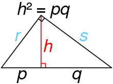
The altitude of a right triangle from its right angle to its hypotenuse is the geometric mean of the lengths of the segments the hypotenuse is split into. Using Pythagoras' theorem on the 3 triangles of sides (p + q, r, s), (r, h, p) and (s, h, q),

{\begin{aligned}(p+q)^{2}\quad &=\quad \;\,r^{2}\quad +\quad s^{2}\\p^{2}\!+2pq+q^{2}&=\left(h^{2}\!\!+\!p^{2}\right)\!+\!\left(h^{2}\!\!+\!q^{2}\right)\\2pq\qquad \,&=2h^{2}\quad \therefore h={\sqrt {pq}}\\\end{aligned}}

In the case of a right triangle, its altitude is the length of a line extending perpendicularly from the hypotenuse to its 90° vertex. Imagining that this line splits the hypotenuse into two segments, the geometric mean of these segment lengths is the length of the altitude. This property is known as the geometric mean theorem.

In an ellipse, the semi-minor axis is the geometric mean of the maximum and minimum distances of the ellipse from a focus; it is also the geometric mean of the semi-major axis and the semi-latus rectum. The semi-major axis of an ellipse is the geometric mean of the distance from the center to either focus and the distance from the center to either directrix.

Distance to the horizon of a sphere is approximately equal to the geometric mean of the distance to the closest point of the sphere and the distance to the farthest point of the sphere when the distance to the closest point of the sphere is small.

Both in the approximation of squaring the circle according to S.A. Ramanujan (1914) and in the construction of the Heptadecagon according to "sent by T. P. Stowell, credited to Leybourn's Math. Repository, 1818", the geometric mean is employed.

Aspect ratios

Equal area comparison of the aspect ratios used by Kerns Powers to derive the SMPTE 16:9 standard.[11] TV 4:3/1.33 in red, 1.66 in orange, 16:9/1.77 in blue, 1.85 in yellow, Panavision/2.2 in mauve and CinemaScope/2.35 in purple.

The geometric mean has been used in choosing a compromise aspect ratio in film and video: given two aspect ratios, the geometric mean of them provides a compromise between them, distorting or cropping both in some sense equally. Concretely, two equal area rectangles (with the same center and parallel sides) of different aspect ratios intersect in a rectangle whose aspect ratio is the geometric mean, and their hull (smallest rectangle which contains both of them) likewise has the aspect ratio of their geometric mean.

In the choice of 16:9 aspect ratio by the SMPTE, balancing 2.35 and 4:3, the geometric mean is ${\textstyle {\sqrt {2.35\times {\frac {4}{3}}}}\approx 1.7701}$ , and thus ${\textstyle 16:9=1.77{\overline {7}}}$ ... was chosen. This was discovered empirically by Kerns Powers, who cut out rectangles with equal areas and shaped them to match each of the popular aspect ratios. When overlapped with their center points aligned, he found that all of those aspect ratio rectangles fit within an outer rectangle with an aspect ratio of 1.77:1 and all of them also covered a smaller common inner rectangle with the same aspect ratio 1.77:1.[11] The value found by Powers is exactly the geometric mean of the extreme aspect ratios, 4:3 (1.33:1) and CinemaScope (2.35:1), which is coincidentally close to ${\textstyle 16:9}$ ( ${\textstyle 1.77{\overline {7}}:1}$ ). The intermediate ratios have no effect on the result, only the two extreme ratios.

Applying the same geometric mean technique to 16:9 and 4:3 approximately yields the 14:9 ( ${\textstyle 1.55{\overline {5}}}$ ...) aspect ratio, which is likewise used as a compromise between these ratios.[12] In this case 14:9 is exactly the arithmetic mean of ${\textstyle 16:9}$ and ${\textstyle 4:3=12:9}$ , since 14 is the average of 16 and 12, while the precise geometric mean is ${\textstyle {\sqrt {{\frac {16}{9}}\times {\frac {4}{3}}}}\approx 1.5396\approx 13.8:9,}$ but the two different means, arithmetic and geometric, are approximately equal because both numbers are sufficiently close to each other (a difference of less than 2%).

Spectral flatness

In signal processing, spectral flatness, a measure of how flat or spiky a spectrum is, is defined as the ratio of the geometric mean of the power spectrum to its arithmetic mean.

Anti-reflective coatings

In optical coatings, where reflection needs to be minimised between two media of refractive indices n₀ and n₂, the optimum refractive index n₁ of the anti-reflective coating is given by the geometric mean: $n_{1}={\sqrt {n_{0}n_{2}}}$ .

Subtractive color mixing

The spectral reflectance curve for paint mixtures (of equal tinting strength, opacity and dilution) is approximately the geometric mean of the paints' individual reflectance curves computed at each wavelength of their spectra.[13]

Image Processing

The geometric mean filter is used as a noise filter in image processing.

Notes and references

Matt Friehauf, Mikaela Hertel, Juan Liu, and Stacey Luong "On Compass and Straightedge Constructions: Means" (PDF). UNIVERSITY of WASHINGTON, DEPARTMENT OF MATHEMATICS. 2013. Retrieved 14 June 2018.
"Euclid, Book VI, Proposition 13". David E. Joyce, Clark University. 2013. Retrieved 19 July 2019.
"TPC-D – Frequently Asked Questions (FAQ)". Transaction Processing Performance Council. Archived from the original on 4 November 2011. Retrieved 9 January 2012.
The geometric mean only applies to numbers of the same sign in order to avoid taking the root of a negative product, which would result in imaginary numbers, and also to satisfy certain properties about means, which is explained later in the article. The definition is unambiguous if one allows 0 (which yields a geometric mean of 0), but may be excluded, as one frequently wishes to take the logarithm of geometric means (to convert between multiplication and addition), and one cannot take the logarithm of 0.
Crawley, Michael J. (2005). Statistics: An Introduction using R. John Wiley & Sons Ltd. ISBN 9780470022986.
Mitchell, Douglas W. (2004). "More on spreads and non-arithmetic means". The Mathematical Gazette. 88: 142–144.
Fleming, Philip J.; Wallace, John J. (1986). "How not to lie with statistics: the correct way to summarize benchmark results". Communications of the ACM. 29 (3): 218–221. doi:10.1145/5666.5673.
Smith, James E. (1988). "Characterizing computer performance with a single number". Communications of the ACM. 31 (10): 1202–1206. doi:10.1145/63039.63043.
Rowley, Eric E. (1987). The Financial System Today. Manchester University Press. ISBN 0719014875.
"Frequently Asked Questions - Human Development Reports". hdr.undp.org. Archived from the original on 2011-03-02.
"TECHNICAL BULLETIN: Understanding Aspect Ratios" (PDF). The CinemaSource Press. 2001. Archived (PDF) from the original on 2009-09-09. Retrieved 2009-10-24. Cite journal requires |journal= (help)
US 5956091, "Method of showing 16:9 pictures on 4:3 displays", issued September 21, 1999
MacEvoy, Bruce. "Colormaking Attributes: Measuring Light & Color". handprint.com/LS/CVS/color.html. Colorimetry. Archived from the original on 2019-07-14. Retrieved 2020-01-02.

External links

This article is issued from Wikipedia. The text is licensed under Creative Commons - Attribution - Sharealike. Additional terms may apply for the media files.

[1] Matt Friehauf, Mikaela Hertel, Juan Liu, and Stacey Luong "On Compass and Straightedge Constructions: Means" (PDF). UNIVERSITY of WASHINGTON, DEPARTMENT OF MATHEMATICS. 2013. Retrieved 14 June 2018.

[2] "Euclid, Book VI, Proposition 13". David E. Joyce, Clark University. 2013. Retrieved 19 July 2019.

[3] "TPC-D – Frequently Asked Questions (FAQ)". Transaction Processing Performance Council. Archived from the original on 4 November 2011. Retrieved 9 January 2012.

[4] The geometric mean only applies to numbers of the same sign in order to avoid taking the root of a negative product, which would result in imaginary numbers, and also to satisfy certain properties about means, which is explained later in the article. The definition is unambiguous if one allows 0 (which yields a geometric mean of 0), but may be excluded, as one frequently wishes to take the logarithm of geometric means (to convert between multiplication and addition), and one cannot take the logarithm of 0.

[5] Crawley, Michael J. (2005). Statistics: An Introduction using R. John Wiley & Sons Ltd. ISBN 9780470022986.

[6] Mitchell, Douglas W. (2004). "More on spreads and non-arithmetic means". The Mathematical Gazette. 88: 142–144.

[7] Fleming, Philip J.; Wallace, John J. (1986). "How not to lie with statistics: the correct way to summarize benchmark results". Communications of the ACM. 29 (3): 218–221. doi:10.1145/5666.5673.

[8] Smith, James E. (1988). "Characterizing computer performance with a single number". Communications of the ACM. 31 (10): 1202–1206. doi:10.1145/63039.63043.

[Rowley_1987-9] Rowley, Eric E. (1987). The Financial System Today. Manchester University Press. ISBN 0719014875.

[10] "Frequently Asked Questions - Human Development Reports". hdr.undp.org. Archived from the original on 2011-03-02.

[Cinemasource-11] "TECHNICAL BULLETIN: Understanding Aspect Ratios" (PDF). The CinemaSource Press. 2001. Archived (PDF) from the original on 2009-09-09. Retrieved 2009-10-24. Cite journal requires |journal= (help)

[12] US 5956091, "Method of showing 16:9 pictures on 4:3 displays", issued September 21, 1999

[13] MacEvoy, Bruce. "Colormaking Attributes: Measuring Light & Color". handprint.com/LS/CVS/color.html. Colorimetry. Archived from the original on 2019-07-14. Retrieved 2020-01-02.