Simple linear regression

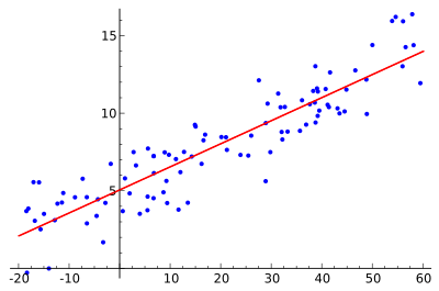
In statistics, simple linear regression is a linear regression model with a single explanatory variable.[1][2][3][4][5] That is, it concerns two-dimensional sample points with one independent variable and one dependent variable (conventionally, the x and y coordinates in a Cartesian coordinate system) and finds a linear function (a non-vertical straight line) that, as accurately as possible, predicts the dependent variable values as a function of the independent variables. The adjective simple refers to the fact that the outcome variable is related to a single predictor.

Okun's law in macroeconomics is an example of the simple linear regression. Here the dependent variable (GDP growth) is presumed to be in a linear relationship with the changes in the unemployment rate.

It is common to make the additional stipulation that the ordinary least squares (OLS) method should be used: the accuracy of each predicted value is measured by its squared residual (vertical distance between the point of the data set and the fitted line), and the goal is to make the sum of these squared deviations as small as possible. Other regression methods that can be used in place of ordinary least squares include least absolute deviations (minimizing the sum of absolute values of residuals) and the Theil–Sen estimator (which chooses a line whose slope is the median of the slopes determined by pairs of sample points). Deming regression (total least squares) also finds a line that fits a set of two-dimensional sample points, but (unlike ordinary least squares, least absolute deviations, and median slope regression) it is not really an instance of simple linear regression, because it does not separate the coordinates into one dependent and one independent variable and could potentially return a vertical line as its fit.

The remainder of the article assumes an ordinary least squares regression. In this case, the slope of the fitted line is equal to the correlation between $y$ and $x$ corrected by the ratio of standard deviations of these variables. The intercept of the fitted line is such that the line passes through the center of mass $(x, y)$ of the data points.

Fitting the regression line

Consider the model function

y=\alpha +\beta x,

which describes a line with slope $β$ and $y$ -intercept $α$ . In general such a relationship may not hold exactly for the largely unobserved population of values of the independent and dependent variables; we call the unobserved deviations from the above equation the errors. Suppose we observe $n$ data pairs and call them ${(x i, y i), i = 1, ..., n$ }. We can describe the underlying relationship between $y i$ and $x i$ involving this error term $ε i$ by

y_{i}=\alpha +\beta x_{i}+\varepsilon _{i}.

This relationship between the true (but unobserved) underlying parameters $α$ and $β$ and the data points is called a linear regression model.

The goal is to find estimated values ${\widehat {\alpha }}$ and ${\widehat {\beta }}$ for the parameters $α$ and $β$ which would provide the "best" fit in some sense for the data points. As mentioned in the introduction, in this article the "best" fit will be understood as in the least-squares approach: a line that minimizes the sum of squared residuals ${\widehat {\varepsilon }}_{i}$ (differences between actual and predicted values of the dependent variable y), each of which is given by, for any candidate parameter values $\alpha$ and $\beta$ ,

{\widehat {\varepsilon }}_{i}=y_{i}-\alpha -\beta x_{i}.

In other words, ${\widehat {\alpha }}$ and ${\widehat {\beta }}$ solve the following minimization problem:

{\text{Find }}\min _{\alpha ,\,\beta }Q(\alpha ,\beta ),\quad {\text{for }}Q(\alpha ,\beta )=\sum _{i=1}^{n}{\widehat {\varepsilon }}_{i}^{\,2}=\sum _{i=1}^{n}(y_{i}-\alpha -\beta x_{i})^{2}\ .

By expanding to get a quadratic expression in $\alpha$ and $\beta ,$ we can derive values of $\alpha$ and $\beta$ that minimize the objective function $Q$ (these minimizing values are denoted ${\widehat {\alpha }}$ and ${\widehat {\beta }}$ ):[6]

{\begin{aligned}{\widehat {\alpha }}&={\bar {y}}-{\widehat {\beta }}\,{\bar {x}},\\[5pt]{\widehat {\beta }}&={\frac {\sum _{i=1}^{n}(x_{i}-{\bar {x}})(y_{i}-{\bar {y}})}{\sum _{i=1}^{n}(x_{i}-{\bar {x}})^{2}}}\\[6pt]&={\frac {s_{x,y}}{s_{x}^{2}}}\\[5pt]&=r_{xy}{\frac {s_{y}}{s_{x}}}.\\[6pt]\end{aligned}}

Here we have introduced

${\bar {x}}$ and ${\bar {y}}$ as the average of the $x i$ and $y i$ , respectively
$r xy$ as the sample correlation coefficient between $x$ and $y$
$s x$ and $s y$ as the uncorrected sample standard deviations of $x$ and $y$
$s_{x}^{2}$ and $s_{x,y}$ as the sample variance and sample covariance, respectively

Substituting the above expressions for ${\widehat {\alpha }}$ and ${\widehat {\beta }}$ into

f={\widehat {\alpha }}+{\widehat {\beta }}x,

yields

{\frac {f-{\bar {y}}}{s_{y}}}=r_{xy}{\frac {x-{\bar {x}}}{s_{x}}}.

This shows that $r xy$ is the slope of the regression line of the standardized data points (and that this line passes through the origin).

Generalizing the ${\bar {x}}$ notation, we can write a horizontal bar over an expression to indicate the average value of that expression over the set of samples. For example:

{\overline {xy}}={\frac {1}{n}}\sum _{i=1}^{n}x_{i}y_{i}.

This notation allows us a concise formula for $r xy$ :

r_{xy}={\frac {{\overline {xy}}-{\bar {x}}{\bar {y}}}{\sqrt {\left({\overline {x^{2}}}-{\bar {x}}^{2}\right)\left({\overline {y^{2}}}-{\bar {y}}^{2}\right)}}}.

The coefficient of determination ("R squared") is equal to $r_{xy}^{2}$ when the model is linear with a single independent variable. See sample correlation coefficient for additional details.

Intuitive explanation

By multiplying all members of the summation in the numerator by : ${\begin{aligned}{\frac {(x_{i}-{\bar {x}})}{(x_{i}-{\bar {x}})}}=1\end{aligned}}$ (thereby not changing it):

{\begin{aligned}{\widehat {\beta }}&={\frac {\sum _{i=1}^{n}(x_{i}-{\bar {x}})(y_{i}-{\bar {y}})}{\sum _{i=1}^{n}(x_{i}-{\bar {x}})^{2}}}={\frac {\sum _{i=1}^{n}(x_{i}-{\bar {x}})^{2}*{\frac {(y_{i}-{\bar {y}})}{(x_{i}-{\bar {x}})}}}{\sum _{i=1}^{n}(x_{i}-{\bar {x}})^{2}}}\\[6pt]\end{aligned}}

We can see that the slope (tangent of angle) of the regression line is the weighted average of ${\frac {(y_{i}-{\bar {y}})}{(x_{i}-{\bar {x}})}}$ that is the slope (tangent of angle) of the line that connects the i-th point to the average of all points, weighted by $(x_{i}-{\bar {x}})^{2}$ because the further the point is the more "important" it is because small errors in its position will affect the slope connecting it to the center point less.

{\begin{aligned}{\widehat {\alpha }}&={\bar {y}}-{\widehat {\beta }}\,{\bar {x}},\\[5pt]\end{aligned}}

Given ${\widehat {\beta }}=\tan(\theta )=dy/dx\rightarrow dy=dx*{\widehat {\beta }}$ with $\theta$ the angle the line makes with the positive x axis, we have $y_{\rm {intersection}}={\bar {y}}-dx*{\widehat {\beta }}={\bar {y}}-dy$

Simple linear regression without the intercept term (single regressor)

Sometimes it is appropriate to force the regression line to pass through the origin, because $x$ and $y$ are assumed to be proportional. For the model without the intercept term, $y = βx$ , the OLS estimator for $β$ simplifies to

{\widehat {\beta }}={\frac {\sum _{i=1}^{n}x_{i}y_{i}}{\sum _{i=1}^{n}x_{i}^{2}}}={\frac {\overline {xy}}{\overline {x^{2}}}}

Substituting $(x - h, y - k)$ in place of $(x, y)$ gives the regression through $(h, k)$ :

{\begin{aligned}{\widehat {\beta }}&={\frac {\overline {(x-h)(y-k)}}{\overline {(x-h)^{2}}}}\\[6pt]&={\frac {{\overline {xy}}-k{\bar {x}}-h{\bar {y}}+hk}{{\overline {x^{2}}}-2h{\bar {x}}+h^{2}}}\\[6pt]&={\frac {{\overline {xy}}-{\bar {x}}{\bar {y}}+({\bar {x}}-h)({\bar {y}}-k)}{{\overline {x^{2}}}-{\bar {x}}^{2}+({\bar {x}}-h)^{2}}}\\[6pt]&={\frac {\operatorname {Cov} (x,y)+({\bar {x}}-h)({\bar {y}}-k)}{\operatorname {Var} (x)+({\bar {x}}-h)^{2}}},\end{aligned}}

where Cov and Var refer to the covariance and variance of the sample data (uncorrected for bias).

The last form above demonstrates how moving the line away from the center of mass of the data points affects the slope.

Numerical properties

The regression line goes through the center of mass point, $({\bar {x}},\,{\bar {y}})$ , if the model includes an intercept term (i.e., not forced through the origin).
The sum of the residuals is zero if the model includes an intercept term:
$\sum _{i=1}^{n}{\widehat {\varepsilon }}_{i}=0.$
The residuals and $x$ values are uncorrelated (whether or not there is an intercept term in the model), meaning:
$\sum _{i=1}^{n}x_{i}{\widehat {\varepsilon }}_{i}\;=\;0$

Model-based properties

Description of the statistical properties of estimators from the simple linear regression estimates requires the use of a statistical model. The following is based on assuming the validity of a model under which the estimates are optimal. It is also possible to evaluate the properties under other assumptions, such as inhomogeneity, but this is discussed elsewhere.

Unbiasedness

The estimators ${\widehat {\alpha }}$ and ${\widehat {\beta }}$ are unbiased.

To formalize this assertion we must define a framework in which these estimators are random variables. We consider the residuals $ε i$ as random variables drawn independently from some distribution with mean zero. In other words, for each value of $x$ , the corresponding value of $y$ is generated as a mean response $α + βx$ plus an additional random variable $ε$ called the error term, equal to zero on average. Under such interpretation, the least-squares estimators ${\widehat {\alpha }}$ and ${\widehat {\beta }}$ will themselves be random variables whose means will equal the "true values" $α$ and $β$ . This is the definition of an unbiased estimator.

Confidence intervals

The formulas given in the previous section allow one to calculate the point estimates of $α$ and $β$ — that is, the coefficients of the regression line for the given set of data. However, those formulas don't tell us how precise the estimates are, i.e., how much the estimators ${\widehat {\alpha }}$ and ${\widehat {\beta }}$ vary from sample to sample for the specified sample size. Confidence intervals were devised to give a plausible set of values to the estimates one might have if one repeated the experiment a very large number of times.

The standard method of constructing confidence intervals for linear regression coefficients relies on the normality assumption, which is justified if either:

the errors in the regression are normally distributed (the so-called classic regression assumption), or
the number of observations $n$ is sufficiently large, in which case the estimator is approximately normally distributed.

The latter case is justified by the central limit theorem.

Normality assumption

Under the first assumption above, that of the normality of the error terms, the estimator of the slope coefficient will itself be normally distributed with mean $β$ and variance $\sigma ^{2}\left/\sum (x_{i}-{\bar {x}})^{2}\right.,$ where $σ 2$ is the variance of the error terms (see Proofs involving ordinary least squares). At the same time the sum of squared residuals $Q$ is distributed proportionally to $χ 2$ with $n - 2$ degrees of freedom, and independently from ${\widehat {\beta }}$ . This allows us to construct a $t$ -value

t={\frac {{\widehat {\beta }}-\beta }{s_{\widehat {\beta }}}}\ \sim \ t_{n-2},

where

s_{\widehat {\beta }}={\sqrt {\frac {{\frac {1}{n-2}}\sum _{i=1}^{n}{\widehat {\varepsilon }}_{i}^{\,2}}{\sum _{i=1}^{n}(x_{i}-{\bar {x}})^{2}}}}

is the standard error of the estimator ${\widehat {\beta }}$ .

This $t$ -value has a Student's $t$ -distribution with $n - 2$ degrees of freedom. Using it we can construct a confidence interval for $β$ :

\beta \in \left[{\widehat {\beta }}-s_{\widehat {\beta }}t_{n-2}^{*},\ {\widehat {\beta }}+s_{\widehat {\beta }}t_{n-2}^{*}\right],

at confidence level $(1 - γ)$ , where $t_{n-2}^{*}$ is the $\scriptstyle \left(1\;-\;{\frac {\gamma }{2}}\right){\text{-th}}$ quantile of the $t n -2$ distribution. For example, if $γ = 0.05$ then the confidence level is 95%.

Similarly, the confidence interval for the intercept coefficient $α$ is given by

\alpha \in \left[{\widehat {\alpha }}-s_{\widehat {\alpha }}t_{n-2}^{*},\ {\widehat {\alpha }}+s_{\widehat {\alpha }}t_{n-2}^{*}\right],

at confidence level (1 − γ), where

s_{\widehat {\alpha }}=s_{\widehat {\beta }}{\sqrt {{\frac {1}{n}}\sum _{i=1}^{n}x_{i}^{2}}}={\sqrt {{\frac {1}{n(n-2)}}\left(\sum _{i=1}^{n}{\widehat {\varepsilon }}_{i}^{\,2}\right){\frac {\sum _{i=1}^{n}x_{i}^{2}}{\sum _{i=1}^{n}(x_{i}-{\bar {x}})^{2}}}}}

The US "changes in unemployment – GDP growth" regression with the 95% confidence bands.

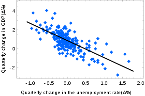
The confidence intervals for $α$ and $β$ give us the general idea where these regression coefficients are most likely to be. For example, in the Okun's law regression shown here the point estimates are

{\widehat {\alpha }}=0.859,\qquad {\widehat {\beta }}=-1.817.

The 95% confidence intervals for these estimates are

\alpha \in \left[\,0.76,0.96\right],\qquad \beta \in \left[-2.06,-1.58\,\right].

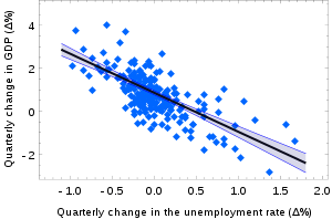
In order to represent this information graphically, in the form of the confidence bands around the regression line, one has to proceed carefully and account for the joint distribution of the estimators. It can be shown[7] that at confidence level (1 − γ) the confidence band has hyperbolic form given by the equation

(\alpha +\beta \xi )\in \left[\,{\widehat {\alpha }}+{\widehat {\beta }}\xi \pm t_{n-2}^{*}{\sqrt {\left({\frac {1}{n-2}}\sum {\widehat {\varepsilon }}_{i}^{\,2}\right)\cdot \left({\frac {1}{n}}+{\frac {(\xi -{\bar {x}})^{2}}{\sum (x_{i}-{\bar {x}})^{2}}}\right)}}\,\right].

Asymptotic assumption

The alternative second assumption states that when the number of points in the dataset is "large enough", the law of large numbers and the central limit theorem become applicable, and then the distribution of the estimators is approximately normal. Under this assumption all formulas derived in the previous section remain valid, with the only exception that the quantile t*_n−2 of Student's t distribution is replaced with the quantile q* of the standard normal distribution. Occasionally the fraction $1 / n -2$ is replaced with $1 / n$ . When $n$ is large such a change does not alter the results appreciably.

Numerical example

This data set gives average masses for women as a function of their height in a sample of American women of age 30–39. Although the OLS article argues that it would be more appropriate to run a quadratic regression for this data, the simple linear regression model is applied here instead.

Height (m), x_i	1.47	1.50	1.52	1.55	1.57	1.60	1.63	1.65	1.68	1.70	1.73	1.75	1.78	1.80	1.83
Mass (kg), y_i	52.21	53.12	54.48	55.84	57.20	58.57	59.93	61.29	63.11	64.47	66.28	68.10	69.92	72.19	74.46

There are n = 15 points in this data set. Hand calculations would be started by finding the following five sums:

{\begin{aligned}&S_{x}=\sum x_{i}=24.76,\quad S_{y}=\sum y_{i}=931.17\\[5pt]&S_{xx}=\sum x_{i}^{2}=41.0532,\quad S_{xy}=\sum x_{i}y_{i}=1548.2453,\quad S_{yy}=\sum y_{i}^{2}=58498.5439\end{aligned}}

These quantities would be used to calculate the estimates of the regression coefficients, and their standard errors.

{\begin{aligned}{\widehat {\beta }}&={\frac {nS_{xy}-S_{x}S_{y}}{nS_{xx}-S_{x}^{2}}}=61.272\\[8pt]{\widehat {\alpha }}&={\frac {1}{n}}S_{y}-{\widehat {\beta }}{\frac {1}{n}}S_{x}=-39.062\\[8pt]s_{\varepsilon }^{2}&={\frac {1}{n(n-2)}}\left[nS_{yy}-S_{y}^{2}-{\widehat {\beta }}^{2}(nS_{xx}-S_{x}^{2})\right]=0.5762\\[8pt]s_{\widehat {\beta }}^{2}&={\frac {ns_{\varepsilon }^{2}}{nS_{xx}-S_{x}^{2}}}=3.1539\\[8pt]s_{\widehat {\alpha }}^{2}&=s_{\widehat {\beta }}^{2}{\frac {1}{n}}S_{xx}=8.63185\end{aligned}}

The 0.975 quantile of Student's t-distribution with 13 degrees of freedom is $t * 13 = 2.1604$ , and thus the 95% confidence intervals for $α$ and $β$ are

{\begin{aligned}&\alpha \in [\,{\widehat {\alpha }}\mp t_{13}^{*}s_{\alpha }\,]=[\,{-45.4},\ {-32.7}\,]\\[5pt]&\beta \in [\,{\widehat {\beta }}\mp t_{13}^{*}s_{\beta }\,]=[\,57.4,\ 65.1\,]\end{aligned}}

The product-moment correlation coefficient might also be calculated:

{\widehat {r}}={\frac {nS_{xy}-S_{x}S_{y}}{\sqrt {(nS_{xx}-S_{x}^{2})(nS_{yy}-S_{y}^{2})}}}=0.9945

This example also demonstrates that sophisticated calculations will not overcome the use of badly prepared data. The heights were originally given in inches, and have been converted to the nearest centimetre. Since the conversion has introduced rounding error, this is not an exact conversion. The original inches can be recovered by Round(x/0.0254) and then re-converted to metric without rounding: if this is done, the results become

{\widehat {\beta }}=61.6746,\qquad {\widehat {\alpha }}=-39.7468.

Thus a seemingly small variation in the data has a real effect.

References

Seltman, Howard J. (2008-09-08). Experimental Design and Analysis (PDF). p. 227.
"Statistical Sampling and Regression: Simple Linear Regression". Columbia University. Retrieved 2016-10-17. When one independent variable is used in a regression, it is called a simple regression;(...)
Lane, David M. Introduction to Statistics (PDF). p. 462.
Zou KH; Tuncali K; Silverman SG (2003). "Correlation and simple linear regression". Radiology. 227 (3): 617–22. doi:10.1148/radiol.2273011499. ISSN 0033-8419. OCLC 110941167. PMID 12773666.
Altman, Naomi; Krzywinski, Martin (2015). "Simple linear regression". Nature Methods. 12 (11): 999–1000. doi:10.1038/nmeth.3627. ISSN 1548-7091. OCLC 5912005539. PMID 26824102.
Kenney, J. F. and Keeping, E. S. (1962) "Linear Regression and Correlation." Ch. 15 in Mathematics of Statistics, Pt. 1, 3rd ed. Princeton, NJ: Van Nostrand, pp. 252–285
Casella, G. and Berger, R. L. (2002), "Statistical Inference" (2nd Edition), Cengage, ISBN 978-0-534-24312-8, pp. 558–559.

External links

This article is issued from Wikipedia. The text is licensed under Creative Commons - Attribution - Sharealike. Additional terms may apply for the media files.

[1] Seltman, Howard J. (2008-09-08). Experimental Design and Analysis (PDF). p. 227.

[:0-2] "Statistical Sampling and Regression: Simple Linear Regression". Columbia University. Retrieved 2016-10-17. When one independent variable is used in a regression, it is called a simple regression;(...)

[3] Lane, David M. Introduction to Statistics (PDF). p. 462.

[4] Zou KH; Tuncali K; Silverman SG (2003). "Correlation and simple linear regression". Radiology. 227 (3): 617–22. doi:10.1148/radiol.2273011499. ISSN 0033-8419. OCLC 110941167. PMID 12773666.

[5] Altman, Naomi; Krzywinski, Martin (2015). "Simple linear regression". Nature Methods. 12 (11): 999–1000. doi:10.1038/nmeth.3627. ISSN 1548-7091. OCLC 5912005539. PMID 26824102.

[6] Kenney, J. F. and Keeping, E. S. (1962) "Linear Regression and Correlation." Ch. 15 in Mathematics of Statistics, Pt. 1, 3rd ed. Princeton, NJ: Van Nostrand, pp. 252–285

[7] Casella, G. and Berger, R. L. (2002), "Statistical Inference" (2nd Edition), Cengage, ISBN 978-0-534-24312-8, pp. 558–559.