Skew normal distribution
In probability theory and statistics, the skew normal distribution is a continuous probability distribution that generalises the normal distribution to allow for non-zero skewness.
|
Probability density function  | |||
|
Cumulative distribution function 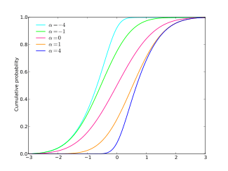 | |||
| Parameters |
location (real) scale (positive, real) shape (real) | ||
|---|---|---|---|
| Support | |||
| CDF |
is Owen's T function | ||
| Mean | where | ||
| Mode | |||
| Variance | |||
| Skewness | |||
| Ex. kurtosis | |||
| MGF | |||
| CF | |||


Definition
Let denote the standard normal probability density function


with the cumulative distribution function given by
- ,

where "erf" is the error function. Then the probability density function (pdf) of the skew-normal distribution with parameter is given by


This distribution was first introduced by O'Hagan and Leonard (1976). Approximations to this distribution that are easier to manipulate mathematically have been given by Ashour and Abdel-Hamid (2010) and by Mudholkar and Hutson (2000).
A stochastic process that underpins the distribution was described by Andel, Netuka and Zvara (1984).[1] Both the distribution and its stochastic process underpinnings were consequences of the symmetry argument developed in Chan and Tong (1986), which applies to multivariate cases beyond normality, e.g. skew multivariate t distribution and others. The distribution is a particular case of a general class of distributions with probability density functions of the form f(x)=2 φ(x) Φ(x) where φ() is any PDF symmetric about zero and Φ() is any CDF whose PDF is symmetric about zero.[2]
To add location and scale parameters to this, one makes the usual transform . One can verify that the normal distribution is recovered when , and that the absolute value of the skewness increases as the absolute value of increases. The distribution is right skewed if and is left skewed if . The probability density function with location , scale , and parameter becomes


Note, however, that the skewness () of the distribution is limited to the interval .


As has been shown [3], the mode (maximum) of the distribution is unique. For general there's no analytic expression for , but a quite accurate (numerical) approximation is:


where and


Estimation
Maximum likelihood estimates for , , and can be computed numerically, but no closed-form expression for the estimates is available unless . If a closed-form expression is needed, the method of moments can be applied to estimate from the sample skew, by inverting the skewness equation. This yields the estimate

where , and is the sample skew. The sign of is the same as the sign of . Consequently, .


The maximum (theoretical) skewness is obtained by setting in the skewness equation, giving . However it is possible that the sample skewness is larger, and then cannot be determined from these equations. When using the method of moments in an automatic fashion, for example to give starting values for maximum likelihood iteration, one should therefore let (for example) .


Concern has been expressed about the impact of skew normal methods on the reliability of inferences based upon them.[4]
Related distributions
The exponentially modified normal distribution is another 3-parameter distribution that is a generalization of the normal distribution to skewed cases. The skew normal still has a normal-like tail in the direction of the skew, with a shorter tail in the other direction; that is, its density is asymptotically proportional to for some positive . Thus, in terms of the seven states of randomness, it shows "proper mild randomness". In contrast, the exponentially modified normal has an exponential tail in the direction of the skew; its density is asymptotically proportional to . In the same terms, it shows "borderline mild randomness".


Thus, the skew normal is useful for modeling skewed distributions which nevertheless have no more outliers than the normal, while the exponentially modified normal is useful for cases with an increased incidence of outliers in (just) one direction.
References
- Andel, J., Netuka, I. and Zvara, K. (1984) On threshold autoregressive processes. Kybernetika, 20, 89-106
- Azzalini, A. (1985). "A class of distributions which includes the normal ones". Scandinavian Journal of Statistics. 12: 171–178.
- Azzalini, Adelchi; Capitanio, Antonella (2014). The skew-normal and related families. pp. 32–33. ISBN 978-1-107-02927-9.
- Pewsey, Arthur. "Problems of inference for Azzalini's skewnormal distribution." Journal of Applied Statistics 27.7 (2000): 859-870
- Andel, J., Netuka, I. and Zvara, K. (1984). On threshold autoregressive processes. Kybernetika, 20, 89-106 .
- Ashour, S., and Abdel-Hamid, M. (2010). Approximate skew normal distribution. Journal of Advanced Research, 1, 341–350.
- Chan, K-S. and Tong, H. (1986). A note on certain integral equations associated with non-linear time series analysis. Probability and Related Fields, 73, 153–158.
- O'Hagan, A. and Leonard, T. (1976). Bayes estimation subject to uncertainty about parameter constraints. Biometrika, 63, 201–202.
- Mudholkar, G. S. and Hutson, A. D. (2000) The epsilon-skew-normal distribution for analyzing near-normal data. Journal of Statistical Planning and Inference, 83, 291–309.
External links
- The multi-variate skew-normal distribution with an application to body mass, height and Body Mass Index
- A very brief introduction to the skew-normal distribution
- The Skew-Normal Probability Distribution (and related distributions, such as the skew-t)
- OWENS: Owen's T Function
- Closed-skew Distributions - Simulation, Inversion and Parameter Estimation