Probability distribution
In probability theory and statistics, a probability distribution is the mathematical function that gives the probabilities of occurrence of different possible outcomes for an experiment.[1][2]
More specifically, the probability distribution is a mathematical description of a random phenomenon in terms of the probabilities of events.[3]
For instance, if the random variable X is used to denote the outcome of a coin toss ("the experiment"), then the probability distribution of X would take the value 0.5 for X = heads, and 0.5 for X = tails (assuming the coin is fair). Examples of random phenomena can include the results of an experiment or survey.
A probability distribution is a mathematical function that has a sample space as its input, and gives a probability as its output. The sample space is the set of all possible outcomes of a random phenomenon being observed; it may be the set of real numbers or a set of vectors, or it may be a list of non-numerical values. For example, the sample space of a coin flip would be {heads, tails} .
Probability distributions are generally divided into two classes. A discrete probability distribution (applicable to the scenarios where the set of possible outcomes is discrete, such as a coin toss or a roll of dice) can be encoded by a discrete list of the probabilities of the outcomes, known as a probability mass function. On the other hand, a continuous probability distribution (applicable to the scenarios where the set of possible outcomes can take on values in a continuous range (e.g. real numbers), such as the temperature on a given day) is typically described by probability density functions (with the probability of any individual outcome actually being 0). The normal distribution is a commonly encountered continuous probability distribution. More complex experiments, such as those involving stochastic processes defined in continuous time, may demand the use of more general probability measures.
A probability distribution whose sample space is one-dimensional (for example real numbers, list of labels, ordered labels or binary) is called univariate, while a distribution whose sample space is a vector space of dimension 2 or more is called multivariate. A univariate distribution gives the probabilities of a single random variable taking on various alternative values; a multivariate distribution (a joint probability distribution) gives the probabilities of a random vector – a list of two or more random variables – taking on various combinations of values. Important and commonly encountered univariate probability distributions include the binomial distribution, the hypergeometric distribution, and the normal distribution. The multivariate normal distribution is a commonly encountered multivariate distribution.
Introduction
.svg.png)
To define probability distributions for the simplest cases, it is necessary to distinguish between discrete and continuous random variables. In the discrete case, it is sufficient to specify a probability mass function assigning a probability to each possible outcome: for example, when throwing a fair die, each of the six values 1 to 6 has the probability 1/6. The probability of an event is then defined to be the sum of the probabilities of the outcomes that satisfy the event; for example, the probability of the event "the dice rolls an even value" is


In contrast, when a random variable takes values from a continuum then typically, any individual outcome has probability zero and only events that include infinitely many outcomes, such as intervals, can have positive probability. For example, the probability that a given object weighs exactly 500 g is zero, because the probability of measuring exactly 500 g tends to zero as the accuracy of our measuring instruments increases. Nevertheless, in quality control one might demand that the probability of a "500 g" package containing between 490 g and 510 g should be no less than 98%, and this demand is less sensitive to the accuracy of measurement instruments.
Continuous probability distributions can be described in several ways. The probability density function describes the infinitesimal probability of any given value, and the probability that the outcome lies in a given interval can be computed by integrating the probability density function over that interval. The probability that the possible values lie in some fixed interval can be related to the way sums converge to an integral; therefore, continuous probability is based on the definition of an integral.
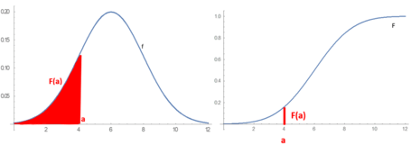
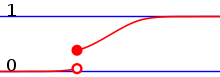
The cumulative distribution function describes the probability that the random variable is no larger than a given value; the probability that the outcome lies in a given interval can be computed by taking the difference between the values of the cumulative distribution function at the endpoints of the interval. The cumulative distribution function is the antiderivative of the probability density function provided that the latter function exists. The cumulative distribution function is the area under the probability density function from minus infinity to as described by the picture to the right.[4]


Terminology[1]
Functions for discrete variables
- Probability function: describes the probability distribution of a discrete random variable
- Probability mass function (PMF): function that gives the probability that a discrete random variable is equal to some value
- Frequency distribution: A table that displays the frequency of various outcomes in a sample.
- Relative frequency distribution: A frequency distribution where each value has been divided (normalized) by a number of outcomes in a sample i.e. sample size.
- Discrete probability distribution function: general term to indicate the way the total probability of 1 is distributed over all various possible outcomes (i.e. over entire population) for discrete random variable
- Cumulative distribution function: function evaluating the probability that will take a value less than or equal to for a discrete random variable
- Categorical distribution: for discrete random variables with a finite set of values.

Functions for continuous variables
- Probability density function (PDF): function whose value at any given sample (or point) in the sample space (the set of possible values taken by the random variable) can be interpreted as providing a relative likelihood that the value of the random variable would equal that sample
- Continuous probability distribution function: most often reserved for continuous random variables
- Cumulative distribution function: function evaluating the probability that will take a value less than or equal to for continuous variable
Basic terms
- Mode: for a discrete random variable, the value with highest probability (the location at which the probability mass function has its peak); for a continuous random variable, a location at which the probability density function has a local peak.
- Support: the smallest closed set whose complement has probability zero.
- Head: the range of values where the pmf or pdf is relatively high.
- Tail: the complement of the head within the support; the large set of values where the pmf or pdf is relatively low.
- Expected value or mean: the weighted average of the possible values, using their probabilities as their weights; or the continuous analog thereof.
- Median: the value such that the set of values less than the median, and the set greater than the median, each have probabilities no greater than one-half.
- Variance: the second moment of the pmf or pdf about the mean; an important measure of the dispersion of the distribution.
- Standard deviation: the square root of the variance, and hence another measure of dispersion.
- Symmetry: a property of some distributions in which the portion of the distribution to the left of a specific value(usually the median) is a mirror image of the portion to its right.
- Skewness: a measure of the extent to which a pmf or pdf "leans" to one side of its mean. The third standardized moment of the distribution.
- Kurtosis: a measure of the "fatness" of the tails of a pmf or pdf. The fourth standardized moment of the distribution.
Cumulative distribution function
Because a probability distribution P on the real line is determined by the probability of a scalar random variable X being in a half-open interval (−∞, x], the probability distribution is completely characterized by its cumulative distribution function:

Discrete probability distribution
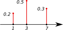

A discrete probability distribution is a probability distribution that can take on a countable number of values.[5] For the probabilities to add up to 1, they have to decline to zero fast enough. For example, if for n = 1, 2, ..., the sum of probabilities would be 1/2 + 1/4 + 1/8 + ... = 1.

Well-known discrete probability distributions used in statistical modeling include the Poisson distribution, the Bernoulli distribution, the binomial distribution, the geometric distribution, and the negative binomial distribution.[3] Additionally, the discrete uniform distribution is commonly used in computer programs that make equal-probability random selections between a number of choices.
When a sample (a set of observations) is drawn from a larger population, the sample points have an empirical distribution that is discrete and that provides information about the population distribution.
Measure theoretic formulation
A measurable function between a probability space and a measurable space is called a discrete random variable provided that its image is a countable set. In this case measurability of means that the pre-images of singleton sets are measurable, i.e., for all . The latter requirement induces a probability mass function via . Since the pre-images of disjoint sets are disjoint,


This recovers the definition given above.
Cumulative distribution function
Equivalently to the above, a discrete random variable can be defined as a random variable whose cumulative distribution function (cdf) increases only by jump discontinuities—that is, its cdf increases only where it "jumps" to a higher value, and is constant between those jumps. Note however that the points where the cdf jumps may form a dense set of the real numbers. The points where jumps occur are precisely the values which the random variable may take.
Delta-function representation
Consequently, a discrete probability distribution is often represented as a generalized probability density function involving Dirac delta functions, which substantially unifies the treatment of continuous and discrete distributions. This is especially useful when dealing with probability distributions involving both a continuous and a discrete part.[6]
Indicator-function representation
For a discrete random variable X, let u0, u1, ... be the values it can take with non-zero probability. Denote

These are disjoint sets, and for such sets

It follows that the probability that X takes any value except for u0, u1, ... is zero, and thus one can write X as

except on a set of probability zero, where is the indicator function of A. This may serve as an alternative definition of discrete random variables.

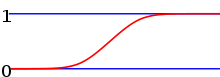
Continuous probability distribution
A continuous probability distribution is a probability distribution with a cumulative distribution function that is absolutely continuous. Equivalently, it is a probability distribution on the real numbers that is absolutely continuous with respect to Lebesgue measure. Such distributions can be represented by their probability density functions. If the distribution of X is continuous, then X is called a continuous random variable. There are many examples of continuous probability distributions: normal, uniform, chi-squared, and others.
Formally, if X is a continuous random variable, then it has a probability density function ƒ(x), and therefore its probability of falling into a given interval, say [a, b], is given by the integral

In particular, the probability for X to take any single value a (that is a ≤ X ≤ a) is zero, because an integral with coinciding upper and lower limits is always equal to zero.
Note on terminology: some authors use the term "continuous distribution" to denote distributions whose cumulative distribution functions are continuous, rather than absolutely continuous. These distributions are the ones such that for all . This definition includes the (absolutely) continuous distributions defined above, but it also includes singular distributions, which are neither absolutely continuous nor discrete nor a mixture of those, and do not have a density. An example is given by the Cantor distribution.


Some properties
- The probability distribution of the sum of two independent random variables is the convolution of each of their distributions.
- Probability distributions are not a vector space—they are not closed under linear combinations, as these do not preserve non-negativity or total integral 1—but they are closed under convex combination, thus forming a convex subset of the space of functions (or measures).
Kolmogorov definition
In the measure-theoretic formalization of probability theory, a random variable is defined as a measurable function from a probability space to a measurable space . Given that probabilities of events of the form satisfy Kolmogorov's probability axioms, the probability distribution of X is the pushforward measure of , which is a probability measure on satisfying .[7][8][9]


Random number generation
Most algorithms are based on a pseudorandom number generator that produces numbers X that are uniformly distributed in the half-open interval [0,1). These random variates X are then transformed via some algorithm to create a new random variate having the required probability distribution. With this source of uniform pseudo-randomness, realizations of any random variable can be generated.[10]
For example, suppose has a uniform distribution between 0 and 1. To construct a random Bernoulli variable for some , we define


so that

This random variable X has a Bernoulli distribution with parameter .[10] Note that this is a transformation of discrete random variable.
For a distribution function of a continuous random variable, a continuous random variable must be constructed. , an inverse function of , relates to the uniform variable :


For example, suppose a random variable that has an exponential distribution must be constructed.


so and if has a distribution, then the random variable is defined by . This has an exponential distribution of .[10]


A frequent problem in statistical simulations (the Monte Carlo method) is the generation of pseudo-random numbers that are distributed in a given way.
Common probability distributions and their applications
The concept of the probability distribution and the random variables which they describe underlies the mathematical discipline of probability theory, and the science of statistics. There is spread or variability in almost any value that can be measured in a population (e.g. height of people, durability of a metal, sales growth, traffic flow, etc.); almost all measurements are made with some intrinsic error; in physics many processes are described probabilistically, from the kinetic properties of gases to the quantum mechanical description of fundamental particles. For these and many other reasons, simple numbers are often inadequate for describing a quantity, while probability distributions are often more appropriate.
The following is a list of some of the most common probability distributions, grouped by the type of process that they are related to. For a more complete list, see list of probability distributions, which groups by the nature of the outcome being considered (discrete, continuous, multivariate, etc.)
All of the univariate distributions below are singly peaked; that is, it is assumed that the values cluster around a single point. In practice, actually observed quantities may cluster around multiple values. Such quantities can be modeled using a mixture distribution.
Linear growth (e.g. errors, offsets)
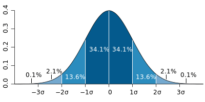
- Normal distribution (Gaussian distribution), for a single such quantity; the most commonly used continuous distribution
Exponential growth (e.g. prices, incomes, populations)
- Log-normal distribution, for a single such quantity whose log is normally distributed
- Pareto distribution, for a single such quantity whose log is exponentially distributed; the prototypical power law distribution
Uniformly distributed quantities
- Discrete uniform distribution, for a finite set of values (e.g. the outcome of a fair die)
- Continuous uniform distribution, for continuously distributed values
Bernoulli trials (yes/no events, with a given probability)
- Basic distributions:
- Bernoulli distribution, for the outcome of a single Bernoulli trial (e.g. success/failure, yes/no)
- Binomial distribution, for the number of "positive occurrences" (e.g. successes, yes votes, etc.) given a fixed total number of independent occurrences
- Negative binomial distribution, for binomial-type observations but where the quantity of interest is the number of failures before a given number of successes occurs
- Geometric distribution, for binomial-type observations but where the quantity of interest is the number of failures before the first success; a special case of the negative binomial distribution
- Related to sampling schemes over a finite population:
- Hypergeometric distribution, for the number of "positive occurrences" (e.g. successes, yes votes, etc.) given a fixed number of total occurrences, using sampling without replacement
- Beta-binomial distribution, for the number of "positive occurrences" (e.g. successes, yes votes, etc.) given a fixed number of total occurrences, sampling using a Pólya urn model (in some sense, the "opposite" of sampling without replacement)
Categorical outcomes (events with K possible outcomes, with a given probability for each outcome)
- Categorical distribution, for a single categorical outcome (e.g. yes/no/maybe in a survey); a generalization of the Bernoulli distribution
- Multinomial distribution, for the number of each type of categorical outcome, given a fixed number of total outcomes; a generalization of the binomial distribution
- Multivariate hypergeometric distribution, similar to the multinomial distribution, but using sampling without replacement; a generalization of the hypergeometric distribution
Poisson process (events that occur independently with a given rate)
- Poisson distribution, for the number of occurrences of a Poisson-type event in a given period of time
- Exponential distribution, for the time before the next Poisson-type event occurs
- Gamma distribution, for the time before the next k Poisson-type events occur
Absolute values of vectors with normally distributed components
- Rayleigh distribution, for the distribution of vector magnitudes with Gaussian distributed orthogonal components. Rayleigh distributions are found in RF signals with Gaussian real and imaginary components.
- Rice distribution, a generalization of the Rayleigh distributions for where there is a stationary background signal component. Found in Rician fading of radio signals due to multipath propagation and in MR images with noise corruption on non-zero NMR signals.
Normally distributed quantities operated with sum of squares (for hypothesis testing)
- Chi-squared distribution, the distribution of a sum of squared standard normal variables; useful e.g. for inference regarding the sample variance of normally distributed samples (see chi-squared test)
- Student's t distribution, the distribution of the ratio of a standard normal variable and the square root of a scaled chi squared variable; useful for inference regarding the mean of normally distributed samples with unknown variance (see Student's t-test)
- F-distribution, the distribution of the ratio of two scaled chi squared variables; useful e.g. for inferences that involve comparing variances or involving R-squared (the squared correlation coefficient)
As a conjugate prior distributions in Bayesian inference
- Beta distribution, for a single probability (real number between 0 and 1); conjugate to the Bernoulli distribution and binomial distribution
- Gamma distribution, for a non-negative scaling parameter; conjugate to the rate parameter of a Poisson distribution or exponential distribution, the precision (inverse variance) of a normal distribution, etc.
- Dirichlet distribution, for a vector of probabilities that must sum to 1; conjugate to the categorical distribution and multinomial distribution; generalization of the beta distribution
- Wishart distribution, for a symmetric non-negative definite matrix; conjugate to the inverse of the covariance matrix of a multivariate normal distribution; generalization of the gamma distribution[11]
Some specialized applications of probability distributions
- The cache language models and other statistical language models used in natural language processing to assign probabilities to the occurrence of particular words and word sequences do so by means of probability distributions.
- In quantum mechanics, the probability density of finding the particle at a given point is proportional to the square of the magnitude of the particle's wavefunction at that point (see Born rule). Therefore, the probability distribution function of the position of a particle is described by , probability that the particle's position x will be in the interval a ≤ x ≤ b in dimension one, and a similar triple integral in dimension three. This is a key principle of quantum mechanics.[12]
- Probabilistic load flow in power-flow study explains the uncertainties of input variables as probability distribution and provide the power flow calculation also in term of probability distribution.[13]
- Prediction of natural phenomena occurrences based on previous frequency distributions such as tropical cyclones, hail, time in between events, etc.[14]

See also
- List of probability distributions
- Copula (statistics)
- Empirical probability
- Histogram
- Joint probability distribution
- Likelihood function
- List of statistical topics
- Kirkwood approximation
- Moment-generating function
- Quasiprobability distribution
- Riemann–Stieltjes integral application to probability theory
References
Citations
- Everitt, Brian. (2006). The Cambridge dictionary of statistics (3rd ed.). Cambridge, UK: Cambridge University Press. ISBN 978-0-511-24688-3. OCLC 161828328.
- Ash, Robert B. (2008). Basic probability theory (Dover ed.). Mineola, N.Y.: Dover Publications. pp. 66–69. ISBN 978-0-486-46628-6. OCLC 190785258.
- Evans, Michael (Michael John) (2010). Probability and statistics : the science of uncertainty. Rosenthal, Jeffrey S. (Jeffrey Seth) (2nd ed.). New York: W.H. Freeman and Co. p. 38. ISBN 978-1-4292-2462-8. OCLC 473463742.
- A modern introduction to probability and statistics : understanding why and how. Dekking, Michel, 1946-. London: Springer. 2005. ISBN 978-1-85233-896-1. OCLC 262680588.CS1 maint: others (link)
- 1941-, Çınlar, E. (Erhan) (2011). Probability and stochastics. New York: Springer. p. 51. ISBN 9780387878591. OCLC 710149819.CS1 maint: numeric names: authors list (link)
- Khuri, André I. (March 2004). "Applications of Dirac's delta function in statistics". International Journal of Mathematical Education in Science and Technology. 35 (2): 185–195. doi:10.1080/00207390310001638313. ISSN 0020-739X.
- W., Stroock, Daniel (1999). Probability theory : an analytic view (Rev. ed.). Cambridge [England]: Cambridge University Press. p. 11. ISBN 978-0521663496. OCLC 43953136.
- Kolmogorov, Andrey (1950) [1933]. Foundations of the theory of probability. New York, USA: Chelsea Publishing Company. pp. 21–24.
- Joyce, David (2014). "Axioms of Probability" (PDF). Clark University. Retrieved December 5, 2019.
- Dekking, Frederik Michel; Kraaikamp, Cornelis; Lopuhaä, Hendrik Paul; Meester, Ludolf Erwin (2005), "Why probability and statistics?", A Modern Introduction to Probability and Statistics, Springer London, pp. 1–11, doi:10.1007/1-84628-168-7_1, ISBN 978-1-85233-896-1
- Bishop, Christopher M. (2006). Pattern recognition and machine learning. New York: Springer. ISBN 0-387-31073-8. OCLC 71008143.
- Chang, Raymond. Physical chemistry for the chemical sciences. Thoman, John W., Jr., 1960-. [Mill Valley, California]. pp. 403–406. ISBN 978-1-68015-835-9. OCLC 927509011.
- Chen, P.; Chen, Z.; Bak-Jensen, B. (April 2008). "Probabilistic load flow: A review". 2008 Third International Conference on Electric Utility Deregulation and Restructuring and Power Technologies. pp. 1586–1591. doi:10.1109/drpt.2008.4523658. ISBN 978-7-900714-13-8.
- Maity, Rajib (2018-04-30). Statistical methods in hydrology and hydroclimatology. Singapore. ISBN 978-981-10-8779-0. OCLC 1038418263.
Sources
- den Dekker, A. J.; Sijbers, J. (2014). "Data distributions in magnetic resonance images: A review". Physica Medica. 30 (7): 725–741. doi:10.1016/j.ejmp.2014.05.002. PMID 25059432.
External links
| Wikimedia Commons has media related to Probability distribution. |
- Hazewinkel, Michiel, ed. (2001) [1994], "Probability distribution", Encyclopedia of Mathematics, Springer Science+Business Media B.V. / Kluwer Academic Publishers, ISBN 978-1-55608-010-4
- Field Guide to Continuous Probability Distributions, Gavin E. Crooks.
Theory of probability distributions | ||
|---|---|---|
 | ||
| ||
| Authority control |
|
|---|