Arithmetic mean
In mathematics and statistics, the arithmetic mean ( /ˌærɪθˈmɛtɪk ˈmiːn/, stress on first and third syllables of "arithmetic"), or simply the mean or average when the context is clear, is the sum of a collection of numbers divided by the count of numbers in the collection.[1] The collection is often a set of results of an experiment or an observational study, or frequently a set of results from a survey. The term "arithmetic mean" is preferred in some contexts in mathematics and statistics because it helps distinguish it from other means, such as the geometric mean and the harmonic mean.
In addition to mathematics and statistics, the arithmetic mean is used frequently in many diverse fields such as economics, anthropology, and history, and it is used in almost every academic field to some extent. For example, per capita income is the arithmetic average income of a nation's population.
While the arithmetic mean is often used to report central tendencies, it is not a robust statistic, meaning that it is greatly influenced by outliers (values that are very much larger or smaller than most of the values). Notably, for skewed distributions, such as the distribution of income for which a few people's incomes are substantially greater than most people's, the arithmetic mean may not coincide with one's notion of "middle", and robust statistics, such as the median, may be a better description of central tendency.
Definition
The arithmetic mean (or mean or average), (read bar), is the mean of the values .[2]


The arithmetic mean is the most commonly used and readily understood measure of central tendency in a data set. In statistics, the term average refers to any of the measures of central tendency. The arithmetic mean of a set of observed data is defined as being equal to the sum of the numerical values of each and every observation divided by the total number of observations. Symbolically, if we have a data set consisting of the values , then the arithmetic mean is defined by the formula:


(See summation for an explanation of the summation operator).
For example, consider the monthly salary of 10 employees of a firm: 2500, 2700, 2400, 2300, 2550, 2650, 2750, 2450, 2600, 2400. The arithmetic mean is

If the data set is a statistical population (i.e., consists of every possible observation and not just a subset of them), then the mean of that population is called the population mean. If the data set is a statistical sample (a subset of the population), we call the statistic resulting from this calculation a sample mean.
The arithmetic mean can be similarly defined for vectors in multiple dimension, not only scalar values; this is often referred to as a centroid. More generally, because the arithmetic mean is a convex combination (coefficients sum to 1), it can be defined on a convex space, not only a vector space.
Motivating properties
The arithmetic mean has several properties that make it useful, especially as a measure of central tendency. These include:
- If numbers have mean , then . Since is the distance from a given number to the mean, one way to interpret this property is as saying that the numbers to the left of the mean are balanced by the numbers to the right of the mean. The mean is the only single number for which the residuals (deviations from the estimate) sum to zero.
- If it is required to use a single number as a "typical" value for a set of known numbers , then the arithmetic mean of the numbers does this best, in the sense of minimizing the sum of squared deviations from the typical value: the sum of . (It follows that the sample mean is also the best single predictor in the sense of having the lowest root mean squared error.)[2] If the arithmetic mean of a population of numbers is desired, then the estimate of it that is unbiased is the arithmetic mean of a sample drawn from the population.


Contrast with median
The arithmetic mean may be contrasted with the median. The median is defined such that no more than half the values are larger than, and no more than half are smaller than, the median. If elements in the data increase arithmetically, when placed in some order, then the median and arithmetic average are equal. For example, consider the data sample . The average is , as is the median. However, when we consider a sample that cannot be arranged so as to increase arithmetically, such as , the median and arithmetic average can differ significantly. In this case, the arithmetic average is 6.2 and the median is 4. In general, the average value can vary significantly from most values in the sample, and can be larger or smaller than most of them.


There are applications of this phenomenon in many fields. For example, since the 1980s, the median income in the United States has increased more slowly than the arithmetic average of income.[3]
Generalizations
Weighted average
A weighted average, or weighted mean, is an average in which some data points count more heavily than others, in that they are given more weight in the calculation. For example, the arithmetic mean of and is , or equivalently . In contrast, a weighted mean in which the first number receives, for example, twice as much weight as the second (perhaps because it is assumed to appear twice as often in the general population from which these numbers were sampled) would be calculated as . Here the weights, which necessarily sum to the value one, are and , the former being twice the latter. The arithmetic mean (sometimes called the "unweighted average" or "equally weighted average") can be interpreted as a special case of a weighted average in which all the weights are equal to each other (equal to in the above example, and equal to in a situation with numbers being averaged).


Continuous probability distributions
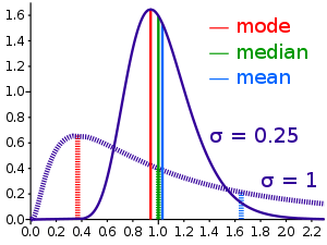
If a numerical property, and any sample of data from it, could take on any value from a continuous range, instead of, for example, just integers, then the probability of a number falling into some range of possible values can be described by integrating a continuous probability distribution across this range, even when the naive probability for a sample number taking one certain value from infinitely many is zero. The analog of a weighted average in this context, in which there are an infinite number of possibilities for the precise value of the variable in each range, is called the mean of the probability distribution. A most widely encountered probability distribution is called the normal distribution; it has the property that all measures of its central tendency, including not just the mean but also the aforementioned median and the mode (the three M's[4]), are equal to each other. This equality does not hold for other probability distributions, as illustrated for the lognormal distribution here.
Angles
Particular care must be taken when using cyclic data, such as phases or angles. Naïvely taking the arithmetic mean of 1° and 359° yields a result of 180°. This is incorrect for two reasons:
- Firstly, angle measurements are only defined up to an additive constant of 360° (or 2π, if measuring in radians). Thus one could as easily call these 1° and −1°, or 361° and 719°, each of which gives a different average.
- Secondly, in this situation, 0° (equivalently, 360°) is geometrically a better average value: there is lower dispersion about it (the points are both 1° from it, and 179° from 180°, the putative average).
In general application, such an oversight will lead to the average value artificially moving towards the middle of the numerical range. A solution to this problem is to use the optimization formulation (viz., define the mean as the central point: the point about which one has the lowest dispersion), and redefine the difference as a modular distance (i.e., the distance on the circle: so the modular distance between 1° and 359° is 2°, not 358°).
Symbols and encoding
The arithmetic mean is often denoted by a bar, for example as in (read bar).[2]
Some software (text processors, web browsers) may not display the x̄ symbol properly. For example, the x̄ symbol in HTML is actually a combination of two codes - the base letter x plus a code for the line above (̄ or ¯).[5]
In some texts, such as pdfs, the x̄ symbol may be replaced by a cent (¢) symbol (Unicode ¢) when copied to text processor such as Microsoft Word.
See also
- Fréchet mean
- Generalized mean
- Geometric mean
- Harmonic mean
- Mode
- Sample mean and covariance
- Standard error of the mean
- Summary statistics
References
- Jacobs, Harold R. (1994). Mathematics: A Human Endeavor (Third ed.). W. H. Freeman. p. 547. ISBN 0-7167-2426-X.
- Medhi, Jyotiprasad (1992). Statistical Methods: An Introductory Text. New Age International. pp. 53–58. ISBN 9788122404197.
- Krugman, Paul (4 June 2014) [Fall 1992]. "The Rich, the Right, and the Facts: Deconstructing the Income Distribution Debate". The American Prospect.
- Thinkmap Visual Thesaurus (30 June 2010). "The Three M's of Statistics: Mode, Median, Mean June 30, 2010". www.visualthesaurus.com. Retrieved 3 December 2018.
- "Notes on Unicode for Stat Symbols". www.personal.psu.edu. Retrieved 14 October 2018.
Further reading
- Huff, Darrell (1993). How to Lie with Statistics. W. W. Norton. ISBN 978-0-393-31072-6.
External links
- Calculations and comparisons between arithmetic mean and geometric mean of two numbers
- Weisstein, Eric W. "Arithmetic Mean". MathWorld.
- Calculate the arithmetic mean of a series of numbers on fxSolver