Generalized gamma distribution
The generalized gamma distribution is a continuous probability distribution with three parameters. It is a generalization of the two-parameter gamma distribution. Since many distributions commonly used for parametric models in survival analysis (such as the Exponential distribution, the Weibull distribution and the Gamma distribution) are special cases of the generalized gamma, it is sometimes used to determine which parametric model is appropriate for a given set of data.[1] Another example is the half-normal distribution.
|
Probability density function 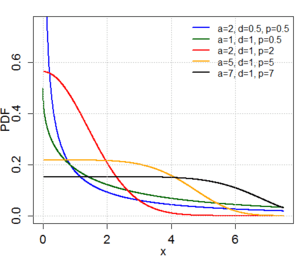 | |||
| Parameters | (scale), | ||
|---|---|---|---|
| Support | |||
| CDF | |||
| Mean | |||
| Mode | |||
| Variance | |||
| Entropy | |||


Characteristics
The generalized gamma has three parameters: , , and . For non-negative x, the probability density function of the generalized gamma is[2]


where denotes the gamma function.

The cumulative distribution function is

where denotes the lower incomplete gamma function.

The quantile function can be found by noting that where is the cumulative distribution function of the Gamma distribution with parameters and . The quantile function is then given by inverting using known relations about inverse of composite functions, yielding:


with being the quantile function for a Gamma distribution with .


If then the generalized gamma distribution becomes the Weibull distribution. Alternatively, if the generalised gamma becomes the gamma distribution.


Alternative parameterisations of this distribution are sometimes used; for example with the substitution α = d/p.[3] In addition, a shift parameter can be added, so the domain of x starts at some value other than zero.[3] If the restrictions on the signs of a, d and p are also lifted (but α = d/p remains positive), this gives a distribution called the Amoroso distribution, after the Italian mathematician and economist Luigi Amoroso who described it in 1925.[4]

Kullback-Leibler divergence
If and are the probability density functions of two generalized gamma distributions, then their Kullback-Leibler divergence is given by


where is the digamma function.[5]

Software implementation
In the R programming language, there are a few packages that include functions for fitting and generating generalized gamma distributions. The gamlss package in r allows for fitting and generating many different distribution families including generalized gamma (family=GG). Other options in R, implemented in the package flexsurv, include the function dgengamma, with parameterization: , , , and in the package ggamma with parametrisation , , .


References
- Box-Steffensmeier, Janet M.; Jones, Bradford S. (2004) Event History Modeling: A Guide for Social Scientists. Cambridge University Press. ISBN 0-521-54673-7 (pp. 41-43)
- Stacy, E.W. (1962). "A Generalization of the Gamma Distribution." Annals of Mathematical Statistics 33(3): 1187-1192. JSTOR 2237889
- Johnson, N.L.; Kotz, S; Balakrishnan, N. (1994) Continuous Univariate Distributions, Volume 1, 2nd Edition. Wiley. ISBN 0-471-58495-9 (Section 17.8.7)
- Gavin E. Crooks (2010), The Amoroso Distribution, Technical Note, Lawrence Berkeley National Laboratory.
- C. Bauckhage (2014), Computing the Kullback-Leibler Divergence between two Generalized Gamma Distributions, arXiv:1401.6853.