Log-normal distribution

Log-normal
	Probability density function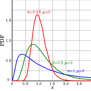; Some log-normal density functions with identical parameter but differing parameters
	Cumulative distribution function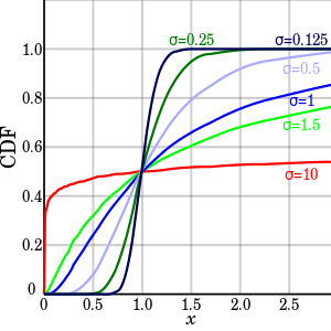; Cumulative distribution function of the log-normal distribution (with )
Notation
Parameters	, ;
Support
PDF
CDF
Mean
Median
Mode
Variance
Skewness
Ex. kurtosis
Entropy
MGF	defined only for numbers with a non-positive real part, see text
CF	representation is asymptotically divergent but sufficient for numerical purposes
Fisher information

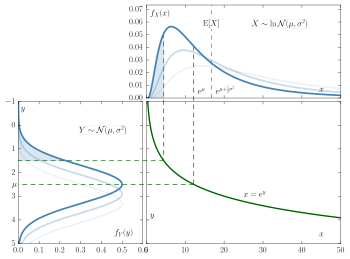
In probability theory, a log-normal (or lognormal) distribution is a continuous probability distribution of a random variable whose logarithm is normally distributed. Thus, if the random variable $X$ is log-normally distributed, then $Y = ln(X)$ has a normal distribution. Likewise, if $Y$ has a normal distribution, then the exponential function of $Y$ , $X = exp(Y)$ , has a log-normal distribution. A random variable which is log-normally distributed takes only positive real values. The distribution is occasionally referred to as the Galton distribution or Galton's distribution, after Francis Galton.^[1] The log-normal distribution also has been associated with other names, such as McAlister, Gibrat and Cobb–Douglas.^[1]

A log-normal process is the statistical realization of the multiplicative product of many independent random variables, each of which is positive. This is justified by considering the central limit theorem in the log domain. The log-normal distribution is the maximum entropy probability distribution for a random variate $X$ for which the mean and variance of $ln(X)$ are specified.^[2]

Notation

Given a log-normally distributed random variable $X$ and two parameters $\mu$ and $\sigma$ that are, respectively, the mean and standard deviation of the variable’s natural logarithm, then the logarithm of $X$ is normally distributed, and we can write $X$ as

X=e^{\mu +\sigma Z}

with $Z$ a standard normal variable.

Relation between normal and lognormal distribution. If

Y=\mu +\sigma Z

is normally distributed, then

X\sim e^{Y}

is lognormally distributed.

This relationship is true regardless of the base of the logarithmic or exponential function. If $\log _{a}(Y)$ is normally distributed, then so is $\log _{b}(Y)$ , for any two positive numbers $a,b\neq 1$ . Likewise, if $e^{X}$ is log-normally distributed, then so is $a^{X}$ , where $a$ is a positive number $\neq 1$ .

The two parameters $\mu$ and $\sigma$ are not location and scale parameters for a lognormally distributed random variable X, but they are respectively location and scale parameters for the normally distributed logarithm ln(X). The quantity e^μ is a scale parameter for the family of lognormal distributions.

In contrast, the mean and variance of the non-logarithmized sample values are respectively denoted $m$ , and $v$ in this article. The two sets of parameters can be related as (see also Arithmetic moments below)^[3]

\mu =\ln \left({\frac {m}{\sqrt {1+{\frac {v}{m^{2}}}}}}\right),\qquad \sigma ^{2}=\ln \left(1+{\frac {v}{m^{2}}}\right).

Characterization

Probability density function

A positive random variable X is log-normally distributed if the logarithm of X is normally distributed,

\ln(X)\sim {\mathcal {N}}(\mu ,\sigma ^{2}).

Let $\Phi$ and $\varphi$ be respectively the cumulative probability distribution function and the probability density function of the N(0,1) distribution.

Then we have^[1]

{\begin{aligned}f_{X}(x)&={\frac {\rm {d}}{{\rm {d}}x}}\Pr(X\leq x)={\frac {\rm {d}}{{\rm {d}}x}}\Pr(\ln X\leq \ln x)\\[6pt]&={\frac {\rm {d}}{{\rm {d}}x}}\Phi \left({\frac {\ln x-\mu }{\sigma }}\right)\\[6pt]&=\varphi \left({\frac {\ln x-\mu }{\sigma }}\right){\frac {\rm {d}}{{\rm {d}}x}}\left({\frac {\ln x-\mu }{\sigma }}\right)\\[6pt]&=\varphi \left({\frac {\ln x-\mu }{\sigma }}\right){\frac {1}{\sigma x}}\\[6pt]&={\frac {1}{x}}\cdot {\frac {1}{\sigma {\sqrt {2\pi \,}}}}\exp \left(-{\frac {(\ln x-\mu )^{2}}{2\sigma ^{2}}}\right).\end{aligned}}

Cumulative distribution function

The cumulative distribution function is

F_{X}(x)=\Phi \left({\frac {(\ln x)-\mu }{\sigma }}\right)

where $\Phi$ is the cumulative distribution function of the standard normal distribution (i.e. N(0,1)).

This may also be expressed as follows:

{\frac {1}{2}}\left[1+\operatorname {erf} \left({\frac {\ln x-\mu }{\sigma {\sqrt {2}}}}\right)\right]={\frac {1}{2}}\operatorname {erfc} \left(-{\frac {\ln x-\mu }{\sigma {\sqrt {2}}}}\right)

where erfc is the complementary error function.

Characteristic function and moment generating function

All moments of the log-normal distribution exist and

\operatorname {E} [X^{n}]=e^{n\mu +n^{2}\sigma ^{2}/2}

This can be derived by letting $z={\frac {\ln(x)-(\mu +n\sigma ^{2})}{\sigma }}$ within the integral. However, the expected value $\operatorname {E} [e^{tX}]$ is not defined for any positive value of the argument $t$ as the defining integral diverges. In consequence the moment generating function is not defined.^[4] The last is related to the fact that the lognormal distribution is not uniquely determined by its moments.

The characteristic function $\operatorname {E} [e^{itX}]$ is defined for real values of $t$ but is not defined for any complex value of $t$ that has a negative imaginary part, and therefore the characteristic function is not analytic at the origin. In consequence, the characteristic function of the log-normal distribution cannot be represented as an infinite convergent series.^[5] In particular, its Taylor formal series diverges:

\sum _{n=0}^{\infty }{\frac {(it)^{n}}{n!}}e^{n\mu +n^{2}\sigma ^{2}/2}

However, a number of alternative divergent series representations have been obtained^[5]^[6]^[7]^[8]

A closed-form formula for the characteristic function $\varphi (t)$ with $t$ in the domain of convergence is not known. A relatively simple approximating formula is available in closed form and given by^[9]

\varphi (t)\approx {\frac {\exp \left(-{\frac {W^{2}(t\sigma ^{2}e^{\mu })+2W(t\sigma ^{2}e^{\mu })}{2\sigma ^{2}}}\right)}{\sqrt {1+W(t\sigma ^{2}e^{\mu })}}}

where $W$ is the Lambert W function. This approximation is derived via an asymptotic method but it stays sharp all over the domain of convergence of $\varphi$ .

Properties

Let $\operatorname {GM} [X]$ denote the geometric mean, and $\operatorname {GSD} [X]$ the geometric standard deviation of the random variable $X$ , and let $\operatorname {E} [X]$ and $\operatorname {SD} [X]$ be the arithmetic mean, or expected value, and the arithmetic standard deviation as usual.

Geometric moments

The geometric mean of the log-normal distribution is $\operatorname {GM} [X]=e^{\mu }$ , and the geometric standard deviation is $\operatorname {GSD} [X]=e^{\sigma }$ .^[10]^[11] By analogy with the arithmetic statistics, one can define a geometric variance, $\operatorname {GVar} [X]=e^{\sigma ^{2}}$ , and a geometric coefficient of variation,^[10] $\operatorname {GCV} [X]=e^{\sigma }-1$ .

Because the log-transformed variable $Y=\ln X$ is symmetric and quantiles are preserved under monotonic transformations, the geometric mean of a log-normal distribution is equal to its median, $\operatorname {Med} [X]$ .^[12]

Note that the geometric mean is less than the arithmetic mean. This is due to the AM–GM inequality, and corresponds to the logarithm being convex down. In fact,

\operatorname {E} [X]=e^{\mu +{\frac {1}{2}}\sigma ^{2}}=e^{\mu }\cdot {\sqrt {e^{\sigma ^{2}}}}=\operatorname {GM} [X]\cdot {\sqrt {\operatorname {GVar} [X]}}.

In finance the term $e^{-{\frac {1}{2}}\sigma ^{2}}$ is sometimes interpreted as a convexity correction. From the point of view of stochastic calculus, this is the same correction term as in Itō's lemma for geometric Brownian motion.

Arithmetic moments

For any real or complex number $n$ , the $n$ -th moment of a log-normally distributed variable $X$ is given by^[1]

\operatorname {E} [X^{n}]=e^{n\mu +{\frac {1}{2}}n^{2}\sigma ^{2}}.

Specifically, the arithmetic mean, expected square, arithmetic variance, and arithmetic standard deviation of a log-normally distributed variable $X$ are given by

{\begin{aligned}&\operatorname {E} [X]=e^{\mu +{\tfrac {1}{2}}\sigma ^{2}},\\&\operatorname {E} [X^{2}]=e^{2\mu +2\sigma ^{2}},\\&\operatorname {Var} [X]=\operatorname {E} [X^{2}]-\operatorname {[} {E}X]^{2}=(\operatorname {E} [X])^{2}(e^{\sigma ^{2}}-1)=e^{2\mu +\sigma ^{2}}(e^{\sigma ^{2}}-1),\\&\operatorname {SD} [X]={\sqrt {\operatorname {Var} [X]}}=\operatorname {E} [X]{\sqrt {e^{\sigma ^{2}}-1}}=e^{\mu +{\tfrac {1}{2}}\sigma ^{2}}{\sqrt {e^{\sigma ^{2}}-1}},\end{aligned}}

respectively.

The parameters $μ$ and $σ$ can be obtained if the arithmetic mean and the arithmetic variance are known:

{\begin{aligned}\mu &=\ln \left({\frac {\operatorname {E} [X]^{2}}{\sqrt {\operatorname {E} [X^{2}]}}}\right)=\ln \left({\frac {\operatorname {E} [X]^{2}}{\sqrt {\operatorname {Var} [X]+\operatorname {E} [X]^{2}}}}\right),\\\sigma ^{2}&=\ln \left({\frac {\operatorname {E} [X^{2}]}{\operatorname {E} [X]^{2}}}\right)=\ln \left(1+{\frac {\operatorname {Var} [X]}{\operatorname {E} [X]^{2}}}\right).\end{aligned}}

A probability distribution is not uniquely determined by the moments $E[X n] = e nμ + 1 / 2 n 2 σ 2$ for $n \geq 1$ . That is, there exist other distributions with the same set of moments.^[1] In fact, there is a whole family of distributions with the same moments as the log-normal distribution.

Mode and median

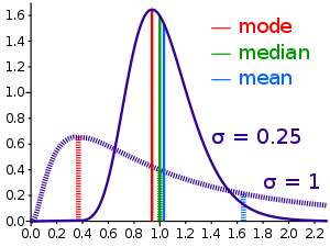
Comparison of mean, median and mode of two log-normal distributions with different skewness.

The mode is the point of global maximum of the probability density function. In particular, it solves the equation $(\ln f)'=0$ :

\operatorname {Mode} [X]=e^{\mu -\sigma ^{2}}.

The median is such a point where $F_{X}=0.5$ :

\operatorname {Med} [X]=e^{\mu }.

Arithmetic coefficient of variation

The arithmetic coefficient of variation $\operatorname {CV} [X]$ is the ratio ${\frac {\operatorname {SD} [X]}{\operatorname {E} [X]}}$ (on the natural scale). For a log-normal distribution it is equal to

\operatorname {CV} [X]={\sqrt {e^{\sigma ^{2}}-1}}.

Contrary to the arithmetic standard deviation, the arithmetic coefficient of variation is independent of the arithmetic mean.

Partial expectation

The partial expectation of a random variable $X$ with respect to a threshold $k$ is defined as

g(k)=\int _{k}^{\infty }xf_{X}(x)\,dx.

Alternatively, and using the definition of conditional expectation, it can be written as $g(k)=\operatorname {E} [X\mid X>k]P(X>k)$ . For a log-normal random variable the partial expectation is given by:

g(k)=\int _{k}^{\infty }xf_{X}(x)\,dx=e^{\mu +{\tfrac {1}{2}}\sigma ^{2}}\,\Phi \!\left({\frac {\mu +\sigma ^{2}-\ln k}{\sigma }}\right)

where Φ is the normal cumulative distribution function. The derivation of the formula is provided in the discussion of this Wikipedia entry. The partial expectation formula has applications in insurance and economics, it is used in solving the partial differential equation leading to the Black–Scholes formula.

Conditional expectation

The conditional expectation of a lognormal random variable $X$ with respect to a threshold $k$ is its partial expectation divided by the cumulative probability of being in that range:

{\begin{aligned}E[X\mid X<k]&=e^{\mu +{\frac {\sigma ^{2}}{2}}}\cdot {\frac {\Phi \left[{\frac {\ln(k)-\mu -\sigma ^{2}}{\sigma }}\right]}{\Phi \left[{\frac {\ln(k)-\mu }{\sigma }}\right]}}\\[8pt]E[X\mid X\geqslant k]&=e^{\mu +{\frac {\sigma ^{2}}{2}}}\cdot {\frac {\Phi \left[{\frac {\mu +\sigma ^{2}-\ln(k)}{\sigma }}\right]}{1-\Phi \left[{\frac {\ln(k)-\mu }{\sigma }}\right]}}\end{aligned}}

Other

A set of data that arises from the log-normal distribution has a symmetric Lorenz curve (see also Lorenz asymmetry coefficient).^[13]

The harmonic $H$ , geometric $G$ and arithmetic $A$ means of this distribution are related;^[14] such relation is given by

H={\frac {G^{2}}{A}}.

Log-normal distributions are infinitely divisible,^[15] but they are not stable distributions, which can be easily drawn from.^[16]

Occurrence and applications

The log-normal distribution is important in the description of natural phenomena. This follows, because many natural growth processes are driven by the accumulation of many small percentage changes. These become additive on a log scale. If the effect of any one change is negligible, the central limit theorem says that the distribution of their sum is more nearly normal than that of the summands. When back-transformed onto the original scale, it makes the distribution of sizes approximately log-normal (though if the standard deviation is sufficiently small, the normal distribution can be an adequate approximation).

This multiplicative version of the central limit theorem is also known as Gibrat's law, after Robert Gibrat (1904–1980) who formulated it for companies.^[17] If the rate of accumulation of these small changes does not vary over time, growth becomes independent of size. Even if that's not true, the size distributions at any age of things that grow over time tends to be log-normal.

Examples include the following:

Human behaviors
- The length of comments posted in Internet discussion forums follows a log-normal distribution.^[18]
- Users' dwell time on online articles (jokes, news etc.) follows a log-normal distribution.^[19]
- The length of chess games tends to follow a log normal distribution.^[20]
- Onset durations of acoustic comparison stimuli that are matched to a standard stimulus follow a log-normal distribution.^[21]
In biology and medicine,
- Measures of size of living tissue (length, skin area, weight);^[22]
- For highly communicable epidemics, such as SARS in 2003, if publication intervention is involved, the number of hospitalized cases is shown to satisfy the lognormal distribution with no free parameters if an entropy is assumed and the standard deviation is determined by the principle of maximum rate of entropy production.
- The length of inert appendages (hair, claws, nails, teeth) of biological specimens, in the direction of growth;
- The normalised RNA-Seq readcount for any genomic region can be well approximated by log-normal distribution.
- Certain physiological measurements, such as blood pressure of adult humans (after separation on male/female subpopulations)^[23]
- In neuroscience, the distribution of firing rates across a population of neurons is often approximately lognormal. This has been first observed in the cortex and striatum ^[24] and later in hippocampus and entorhinal cortex,^[25] and elsewhere in the brain.^[26]^[27] Also, intrinsic gain distributions and synaptic weight distributions appear to be lognormal^[28] as well.

In colloidal chemistry and polymer chemistry
- Particle size distributions
- Molar mass distributions

Consequently, reference ranges for measurements in healthy individuals are more accurately estimated by assuming a log-normal distribution than by assuming a symmetric distribution about the mean.

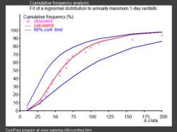
Fitted cumulative log-normal distribution to annually maximum 1-day rainfalls, see distribution fitting

In hydrology, the log-normal distribution is used to analyze extreme values of such variables as monthly and annual maximum values of daily rainfall and river discharge volumes.^[29]

The image on the right, made with CumFreq, illustrates an example of fitting the log-normal distribution to ranked annually maximum one-day rainfalls showing also the 90% confidence belt based on the binomial distribution.^[30]

The rainfall data are represented by plotting positions as part of a cumulative frequency analysis.

In social sciences and demographics
- In economics, there is evidence that the income of 97%–99% of the population is distributed log-normally.^[31] (The distribution of higher-income individuals follows a Pareto distribution.^[32])
- In finance, in particular the Black–Scholes model, changes in the logarithm of exchange rates, price indices, and stock market indices are assumed normal^[33] (these variables behave like compound interest, not like simple interest, and so are multiplicative). However, some mathematicians such as Benoît Mandelbrot have argued ^[34] that log-Lévy distributions, which possesses heavy tails would be a more appropriate model, in particular for the analysis for stock market crashes. Indeed, stock price distributions typically exhibit a fat tail.;^[35] the fat tailed distribution of changes during stock market crashes invalidate the assumptions of the central limit theorem.
- In scientometrics, the number of citations to journal articles and patents follows a discrete log-normal distribution.^[36]
- City sizes.
Technology
- In reliability analysis, the lognormal distribution is often used to model times to repair a maintainable system.^[37]
- In wireless communication, "the local-mean power expressed in logarithmic values, such as dB or neper, has a normal (i.e., Gaussian) distribution." ^[38] Also, the random obstruction of radio signals due to large buildings and hills, called shadowing, is often modeled as a lognormal distribution.
- Particle size distributions produced by comminution with random impacts, such as in ball milling
- The file size distribution of publicly available audio and video data files (MIME types) follows a log-normal distribution over five orders of magnitude.^[39]

Extremal principle of entropy to fix the free parameter $\sigma$

In applications, $\sigma$ is a parameter to be determined. In cases that there are no data to determine this parameter, it is possible to evaluate it from some universal principle. One is the entropy method. For growing processes which are governed by production and dissipation, it was shown that one can use some extremal principle of Shannon entropy to determine this parameter to be $\sigma =1{\big /}{\sqrt {6}}$ . This value can then be used to give some scaling relation between the inflexion point and maximum point of the lognormal distribution.^[40] It is shown that this relationship is determined by the base of natural logarithm, $e=2.718\ldots$ , and exhibits some geometrical similarity to the minimal surface energy principle. These scaling relations are shown to be useful for predicting a number of growth processes (epidemic spreading, droplet splashing, population growth, swirling rate of the bathtub vortex, distribution of language characters, velocity profile of turbulences, etc.). For instance, the lognormal function with such $\sigma$ fits well with the size of secondary produced droplet during droplet impact ^[41] and the spreading of one epidemic disease.^[42]

Maximum likelihood estimation of parameters

For determining the maximum likelihood estimators of the log-normal distribution parameters μ and σ, we can use the same procedure as for the normal distribution. To avoid repetition, we observe that

L(\mu ,\sigma )=\prod _{i=1}^{n}{\frac {1}{x_{i}}}\varphi _{\mu ,\sigma }(\ln x_{i})

where $\varphi _{}$ is the density function of the normal distribution ${\mathcal {N}}(\mu ,\sigma ^{2})$ . Therefore, using the same indices to denote distributions, we can write the log-likelihood function thus:

{\begin{aligned}\ell (\mu ,\sigma \mid x_{1},x_{2},\ldots ,x_{n})&=-\sum _{k}\ln x_{k}+\ell _{N}(\mu ,\sigma \mid \ln x_{1},\ln x_{2},\dots ,\ln x_{n})\\&={\text{constant}}+\ell _{N}(\mu ,\sigma \mid \ln x_{1},\ln x_{2},\dots ,\ln x_{n}).\end{aligned}}

Since the first term is constant with regard to μ and σ, both logarithmic likelihood functions, $\ell _{L}$ and $\ell _{N}$ , reach their maximum with the same $\mu$ and $\sigma$ . Hence, using the formulas for the normal distribution maximum likelihood parameter estimators and the equality above, we deduce that for the log-normal distribution it holds that

{\widehat {\mu }}={\frac {\sum _{k}\ln x_{k}}{n}},\qquad {\widehat {\sigma }}^{2}={\frac {\sum _{k}\left(\ln x_{k}-{\widehat {\mu }}\right)^{2}}{n}}.

Multivariate log-normal

If ${\boldsymbol {X}}\sim {\mathcal {N}}({\boldsymbol {\mu }},\,{\boldsymbol {\Sigma }})$ is a multivariate normal distribution then ${\boldsymbol {Y}}=\exp({\boldsymbol {X}})$ has a multivariate log-normal distribution^[43]^[44] with mean

\operatorname {E} [{\boldsymbol {Y}}]_{i}=e^{\mu _{i}+{\frac {1}{2}}\Sigma _{ii}},

and covariance matrix

\operatorname {Var} [{\boldsymbol {Y}}]_{ij}=e^{\mu _{i}+\mu _{j}+{\frac {1}{2}}(\Sigma _{ii}+\Sigma _{jj})}(e^{\Sigma _{ij}}-1).

Related distributions

If $X\sim {\mathcal {N}}(\mu ,\sigma ^{2})$ is a normal distribution, then $\exp(X)\sim \operatorname {Lognormal} (\mu ,\sigma ^{2}).$
If $X\sim \operatorname {Lognormal} (\mu ,\sigma ^{2})$ is distributed log-normally, then $\ln(X)\sim {\mathcal {N}}(\mu ,\sigma ^{2})$ is a normal random variable.
If $X_{j}\sim \operatorname {Lognormal} (\mu _{j},\sigma _{j}^{2})$ are $n$ independent log-normally distributed variables, and $Y=\textstyle \prod _{j=1}^{n}X_{j}$ , then $Y$ is also distributed log-normally:

Y\sim \operatorname {Lognormal} {\Big (}\textstyle \sum _{j=1}^{n}\mu _{j},\ \sum _{j=1}^{n}\sigma _{j}^{2}{\Big )}.

Let $X_{j}\sim \operatorname {Lognormal} (\mu _{j},\sigma _{j}^{2})\$ be independent log-normally distributed variables with possibly varying $\sigma$ and $\mu$ parameters, and $Y=\textstyle \sum _{j=1}^{n}X_{j}$ . The distribution of $Y$ has no closed-form expression, but can be reasonably approximated by another log-normal distribution $Z$ at the right tail.^[45] Its probability density function at the neighborhood of 0 has been characterized^[16] and it does not resemble any log-normal distribution. A commonly used approximation due to L.F. Fenton (but previously stated by R.I. Wilkinson and mathematical justified by Marlow^[46]) is obtained by matching the mean and variance of another lognormal distribution:

{\begin{aligned}\sigma _{Z}^{2}&=\ln \!\left[{\frac {\sum e^{2\mu _{j}+\sigma _{j}^{2}}(e^{\sigma _{j}^{2}}-1)}{(\sum e^{\mu _{j}+\sigma _{j}^{2}/2})^{2}}}+1\right],\\\mu _{Z}&=\ln \!\left[\sum e^{\mu _{j}+\sigma _{j}^{2}/2}\right]-{\frac {\sigma _{Z}^{2}}{2}}.\end{aligned}}

In the case that all

X_{j}

have the same variance parameter

\sigma _{j}=\sigma

, these formulas simplify to

{\begin{aligned}\sigma _{Z}^{2}&=\ln \!\left[(e^{\sigma ^{2}}-1){\frac {\sum e^{2\mu _{j}}}{(\sum e^{\mu _{j}})^{2}}}+1\right],\\\mu _{Z}&=\ln \!\left[\sum e^{\mu _{j}}\right]+{\frac {\sigma ^{2}}{2}}-{\frac {\sigma _{Z}^{2}}{2}}.\end{aligned}}

For a more accurate approximation one can use the Monte Carlo method to estimate the cumulative distribution function, the pdf and right tail. ^[47] ^[48]

If $X\sim \operatorname {Lognormal} (\mu ,\sigma ^{2})$ then $X+c$ is said to have a shifted log-normal distribution with support $x\in (c,+\infty )$ . $\operatorname {E} [X+c]=\operatorname {E} [X]+c$ , $\operatorname {Var} [X+c]=\operatorname {Var} [X]$ .
If $X\sim \operatorname {Lognormal} (\mu ,\sigma ^{2})$ then $aX\sim \operatorname {Lognormal} (\mu +\ln a,\ \sigma ^{2}).$
If $X\sim \operatorname {Lognormal} (\mu ,\sigma ^{2})$ then ${\tfrac {1}{X}}\sim \operatorname {Lognormal} (-\mu ,\ \sigma ^{2}).$
If $X\sim \operatorname {Lognormal} (\mu ,\sigma ^{2})$ then $X^{a}\sim \operatorname {Lognormal} (a\mu ,\ a^{2}\sigma ^{2})$ for $a\neq 0.$
Lognormal distribution is a special case of semi-bounded Johnson distribution
If $X\mid Y\sim \operatorname {Rayleigh} (Y)\,$ with $Y\sim \operatorname {Lognormal} (\mu ,\sigma ^{2})$ , then $X\sim \operatorname {Suzuki} (\mu ,\sigma )$ (Suzuki distribution)
A substitute for the log-normal whose integral can be expressed in terms of more elementary functions^[49] can be obtained based on the logistic distribution to get an approximation for the CDF

F(x;\mu ,\sigma )=\left[\left({\frac {e^{\mu }}{x}}\right)^{\pi /(\sigma {\sqrt {3}})}+1\right]^{-1}.

This is a log-logistic distribution.

Notes

1 2 3 4 5 Johnson, Norman L.; Kotz, Samuel; Balakrishnan, N. (1994), "14: Lognormal Distributions", Continuous univariate distributions. Vol. 1, Wiley Series in Probability and Mathematical Statistics: Applied Probability and Statistics (2nd ed.), New York: John Wiley & Sons, ISBN 978-0-471-58495-7, MR 1299979
↑ Park, Sung Y.; Bera, Anil K. (2009). "Maximum entropy autoregressive conditional heteroskedasticity model" (PDF). Journal of Econometrics. Elsevier. 150 (2): 219–230. doi:10.1016/j.jeconom.2008.12.014. Retrieved 2011-06-02. Table 1, p. 221.
↑ "Lognormal mean and variance - MATLAB lognstat". www.mathworks.com. Retrieved 14 April 2018.
↑ Heyde, CC. (1963), "On a property of the lognormal distribution", Journal of the Royal Statistical Society, Series B, 25 (2): 392–393, doi:10.1007/978-1-4419-5823-5_6
1 2 Holgate, P. (1989). "The lognormal characteristic function, vol. 18, pp. 4539–4548, 1989". Communications in Statistical – Theory and Methods. 18 (12): 4539–4548. doi:10.1080/03610928908830173.
↑ Barakat, R. (1976). "Sums of independent lognormally distributed random variables". Journal of the Optical Society of America. 66 (3): 211–216. doi:10.1364/JOSA.66.000211.
↑ Barouch, E.; Kaufman, GM.; Glasser, ML. (1986). "On sums of lognormal random variables" (PDF). Studies in Applied Mathematics. 75 (1): 37–55.
↑ Leipnik, Roy B. (January 1991). "On Lognormal Random Variables: I – The Characteristic Function". Journal of the Australian Mathematical Society Series B. 32 (3): 327–347. doi:10.1017/S0334270000006901.
↑ S. Asmussen, J.L. Jensen, L. Rojas-Nandayapa (2016). "On the Laplace transform of the Lognormal distribution", Methodology and Computing in Applied Probability 18 (2), 441-458. Thiele report 6 (13).
1 2 Kirkwood, Thomas BL (Dec 1979). "Geometric means and measures of dispersion". Biometrics. 35 (4): 908–9. doi:10.2307/2530139.
↑ Limpert, E; Stahel, W; Abbt, M (2001). "Lognormal distributions across the sciences: keys and clues". BioScience. 51 (5): 341–352. doi:10.1641/0006-3568(2001)051[0341:LNDATS]2.0.CO;2.
↑ Daly, Leslie E.; Bourke, Geoffrey Joseph (2000). Interpretation and uses of medical statistics (5th ed.). Wiley-Blackwell. p. 89. doi:10.1002/9780470696750. ISBN 978-0-632-04763-5.
↑ Damgaard, Christian; Weiner, Jacob (2000). "Describing inequality in plant size or fecundity". Ecology. 81 (4): 1139–1142. doi:10.1890/0012-9658(2000)081[1139:DIIPSO]2.0.CO;2.
↑ Rossman, Lewis A (July 1990). "Design stream ﬂows based on harmonic means". J Hydraulic Engineering. 116 (7): 946–950. doi:10.1061/(ASCE)0733-9429(1990)116:7(946).
↑ Thorin, Olof (1977). "On the infinite divisibility of the lognormal distribution". Scandinavian Actuarial Journal. 1977 (3): 121–148. doi:10.1080/03461238.1977.10405635. ISSN 0346-1238.
1 2 Gao, Xin (2009). "Asymptotic Behavior of Tail Density for Sum of Correlated Lognormal Variables". International Journal of Mathematics and Mathematical Sciences. 2009: 1–28. doi:10.1155/2009/630857.
↑ Sutton, John (Mar 1997). "Gibrat's Legacy". Journal of Economic Literature. 32 (1): 40–59. JSTOR 2729692.
↑ Pawel, Sobkowicz; et al. (2013). "Lognormal distributions of user post lengths in Internet discussions - a consequence of the Weber-Fechner law?". EPJ Data Science.
↑ Yin, Peifeng; Luo, Ping; Lee, Wang-Chien; Wang, Min (2013). Silence is also evidence: interpreting dwell time for recommendation from psychological perspective. ACM International Conference on KDD.
↑ "What is the average length of a game of chess?". chess.stackexchange.com. Retrieved 14 April 2018.
↑ Heil P, Friedrich B (2017). "Onset-Duration Matching of Acoustic Stimuli Revisited: Conventional Arithmetic vs. Proposed Geometric Measures of Accuracy and Precision". Frontiers in Psychology. 7: 2013. doi:10.3389/fpsyg.2016.02013.
↑ Huxley, Julian S. (1932). Problems of relative growth. London. ISBN 0-486-61114-0. OCLC 476909537.
↑ Makuch, Robert W.; D.H. Freeman; M.F. Johnson (1979). "Justification for the lognormal distribution as a model for blood pressure". Journal of Chronic Diseases. 32 (3): 245–250. doi:10.1016/0021-9681(79)90070-5. Retrieved 27 February 2012.
↑ Scheler, Gabriele; Schumann, Johann (2006-10-08). Diversity and stability in neuronal output rates. 36th Society for Neuroscience Meeting, Atlanta.
↑ Mizuseki, Kenji; Buzsáki, György (2013-09-12). "Preconfigured, skewed distribution of firing rates in the hippocampus and entorhinal cortex". Cell Reports. 4 (5): 1010–1021. doi:10.1016/j.celrep.2013.07.039. ISSN 2211-1247. PMC 3804159. PMID 23994479.
↑ Buzsáki, György; Mizuseki, Kenji (2017-01-06). "The log-dynamic brain: how skewed distributions affect network operations". Nature Reviews. Neuroscience. 15 (4): 264–278. doi:10.1038/nrn3687. ISSN 1471-003X. PMC 4051294. PMID 24569488.
↑ Wohrer, Adrien; Humphries, Mark D.; Machens, Christian K. (2013-04-01). "Population-wide distributions of neural activity during perceptual decision-making". Progress in Neurobiology. 103: 156–193. doi:10.1016/j.pneurobio.2012.09.004. ISSN 1873-5118. PMID 23123501.
↑ Scheler, Gabriele (2017-07-28). "Logarithmic distributions prove that intrinsic learning is Hebbian". F1000research. 6: 1222. doi:10.12688/f1000research.12130.2. PMC 5639933. PMID 29071065.
↑ Ritzema (ed.), H.P. (1994). Frequency and Regression Analysis (PDF). Chapter 6 in: Drainage Principles and Applications, Publication 16, International Institute for Land Reclamation and Improvement (ILRI), Wageningen, The Netherlands. pp. 175–224. ISBN 90-70754-33-9.
↑ CumFreq, free software for distribution fitting
↑ Clementi, Fabio; Gallegati, Mauro (2005) "Pareto's law of income distribution: Evidence for Germany, the United Kingdom, and the United States", EconWPA
↑ Wataru, Souma (2002-02-22). "Physics of Personal Income". arXiv:cond-mat/0202388. Bibcode:2002cond.mat..2388S.
↑ Black, F.; Scholes, M. (1973). "The Pricing of Options and Corporate Liabilities". Journal of Political Economy. 81 (3): 637. doi:10.1086/260062.
↑ Mandelbrot, Benoit (2004). The (mis-)Behaviour of Markets. Basic Books. ISBN 9780465043552.
↑ Bunchen, P., Advanced Option Pricing, University of Sydney coursebook, 2007
↑ Thelwall, Mike; Wilson, Paul (2014). "Regression for citation data: An evaluation of different methods". Journal of Infometrics. 8 (4): 963–971.
↑ O'Connor, Patrick; Kleyner, Andre (2011). Practical Reliability Engineering. John Wiley & Sons. p. 35. ISBN 978-0-470-97982-2.
↑ http://wireless.per.nl/reference/chaptr03/shadow/shadow.htm Archived January 13, 2012, at the Wayback Machine.
↑ Gros, C; Kaczor, G.; Markovic, D (2012). "Neuropsychological constraints to human data production on a global scale". The European Physical Journal B. 85 (28). arXiv:1111.6849. Bibcode:2012EPJB...85...28G. doi:10.1140/epjb/e2011-20581-3.
↑ Wu, Ziniu; Li, Juan; Bai, Chenyuan (2017). "Scaling Relations of Lognormal Type Growth Process with an Extremal Principle of Entropy". Entropy. 19 (56): 1–14. Bibcode:2017Entrp..19...56W. doi:10.3390/e19020056.
↑ Wu, Zi-Niu (2003). "Prediction of the size distribution of secondary ejected droplets by crown splashing of droplets impinging on a solid wall". Probabilistic Engineering Mechanics. 18: 241–249. doi:10.1016/S0266-8920(03)00028-6.
↑ Wang, WenBin; Wu, ZiNiu; Wang, ChunFeng; Hu, RuiFeng (2013). "Modelling the spreading rate of controlled communicable epidemics through an entropy-based thermodynamic model". Science China Physics, Mechanics and Astronomy. 56 (11): 2143–2150. arXiv:1304.5603. Bibcode:2013SCPMA..56.2143W. doi:10.1007/s11433-013-5321-0. ISSN 1674-7348.
↑ Tarmast, Ghasem (2001). Multivariate Log–Normal Distribution (PDF). ISI Proceedings: 53rd Session. Seoul.
↑ Halliwell, Leigh (2015). The Lognormal Random Multivariate (PDF). Casualty Actuarial Society E-Forum, Spring 2015. Arlington, VA.
↑ Asmussen, S.; Rojas-Nandayapa, L. (2008). "Asymptotics of Sums of Lognormal Random Variables with Gaussian Copula". Statistics and Probability Letters. 78 (16): 2709–2714. doi:10.1016/j.spl.2008.03.035.
↑ Marlow, NA. (Nov 1967). "A normal limit theorem for power sums of independent normal random variables". Bell System Technical Journal. 46 (9): 2081–2089. doi:10.1002/j.1538-7305.1967.tb04244.x.
↑ Botev, Z. I.; L'Ecuyer, P. (2017). "Accurate computation of the right tail of the sum of dependent log-normal variates". 2017 Winter Simulation Conference (WSC). 3th–6th Dec 2017 Las Vegas, NV, USA: IEEE. pp. 1880–1890. arXiv:1705.03196. doi:10.1109/WSC.2017.8247924. ISBN 978-1-5386-3428-8.
↑ Asmussen, A.; Goffard, P.-O.; Laub, P. J. (2016). "Orthonormal polynomial expansions and lognormal sum densities". arXiv:1601.01763v1.
↑ Swamee, P. K. (2002). "Near Lognormal Distribution". Journal of Hydrologic Engineering. 7 (6): 441–444. doi:10.1061/(ASCE)1084-0699(2002)7:6(441).

External links

This article is issued from Wikipedia. The text is licensed under Creative Commons - Attribution - Sharealike. Additional terms may apply for the media files.

[JKB-1] 1 2 3 4 5 Johnson, Norman L.; Kotz, Samuel; Balakrishnan, N. (1994), "14: Lognormal Distributions", Continuous univariate distributions. Vol. 1, Wiley Series in Probability and Mathematical Statistics: Applied Probability and Statistics (2nd ed.), New York: John Wiley & Sons, ISBN 978-0-471-58495-7, MR 1299979

[2] Park, Sung Y.; Bera, Anil K. (2009). "Maximum entropy autoregressive conditional heteroskedasticity model" (PDF). Journal of Econometrics. Elsevier. 150 (2): 219–230. doi:10.1016/j.jeconom.2008.12.014. Retrieved 2011-06-02. Table 1, p. 221.

[3] "Lognormal mean and variance - MATLAB lognstat". www.mathworks.com. Retrieved 14 April 2018.

[Heyde-4] Heyde, CC. (1963), "On a property of the lognormal distribution", Journal of the Royal Statistical Society, Series B, 25 (2): 392–393, doi:10.1007/978-1-4419-5823-5_6

[Holgate-5] 1 2 Holgate, P. (1989). "The lognormal characteristic function, vol. 18, pp. 4539–4548, 1989". Communications in Statistical – Theory and Methods. 18 (12): 4539–4548. doi:10.1080/03610928908830173.

[Barakat-6] Barakat, R. (1976). "Sums of independent lognormally distributed random variables". Journal of the Optical Society of America. 66 (3): 211–216. doi:10.1364/JOSA.66.000211.

[Barouch-7] Barouch, E.; Kaufman, GM.; Glasser, ML. (1986). "On sums of lognormal random variables" (PDF). Studies in Applied Mathematics. 75 (1): 37–55.

[Leipnik-8] Leipnik, Roy B. (January 1991). "On Lognormal Random Variables: I – The Characteristic Function". Journal of the Australian Mathematical Society Series B. 32 (3): 327–347. doi:10.1017/S0334270000006901.

[Asmussen-9] S. Asmussen, J.L. Jensen, L. Rojas-Nandayapa (2016). "On the Laplace transform of the Lognormal distribution", Methodology and Computing in Applied Probability 18 (2), 441-458. Thiele report 6 (13).

[ReferenceA-10] 1 2 Kirkwood, Thomas BL (Dec 1979). "Geometric means and measures of dispersion". Biometrics. 35 (4): 908–9. doi:10.2307/2530139.

[11] Limpert, E; Stahel, W; Abbt, M (2001). "Lognormal distributions across the sciences: keys and clues". BioScience. 51 (5): 341–352. doi:10.1641/0006-3568(2001)051[0341:LNDATS]2.0.CO;2.

[12] Daly, Leslie E.; Bourke, Geoffrey Joseph (2000). Interpretation and uses of medical statistics (5th ed.). Wiley-Blackwell. p. 89. doi:10.1002/9780470696750. ISBN 978-0-632-04763-5.

[EcolgyArticle-13] Damgaard, Christian; Weiner, Jacob (2000). "Describing inequality in plant size or fecundity". Ecology. 81 (4): 1139–1142. doi:10.1890/0012-9658(2000)081[1139:DIIPSO]2.0.CO;2.

[Rossman1990-14] Rossman, Lewis A (July 1990). "Design stream ﬂows based on harmonic means". J Hydraulic Engineering. 116 (7): 946–950. doi:10.1061/(ASCE)0733-9429(1990)116:7(946).

[OlofThorin1978LNInfDivi-15] Thorin, Olof (1977). "On the infinite divisibility of the lognormal distribution". Scandinavian Actuarial Journal. 1977 (3): 121–148. doi:10.1080/03461238.1977.10405635. ISSN 0346-1238.

[Gao-16] 1 2 Gao, Xin (2009). "Asymptotic Behavior of Tail Density for Sum of Correlated Lognormal Variables". International Journal of Mathematics and Mathematical Sciences. 2009: 1–28. doi:10.1155/2009/630857.

[17] Sutton, John (Mar 1997). "Gibrat's Legacy". Journal of Economic Literature. 32 (1): 40–59. JSTOR 2729692.

[18] Pawel, Sobkowicz; et al. (2013). "Lognormal distributions of user post lengths in Internet discussions - a consequence of the Weber-Fechner law?". EPJ Data Science.

[19] Yin, Peifeng; Luo, Ping; Lee, Wang-Chien; Wang, Min (2013). Silence is also evidence: interpreting dwell time for recommendation from psychological perspective. ACM International Conference on KDD.

[20] "What is the average length of a game of chess?". chess.stackexchange.com. Retrieved 14 April 2018.

[21] Heil P, Friedrich B (2017). "Onset-Duration Matching of Acoustic Stimuli Revisited: Conventional Arithmetic vs. Proposed Geometric Measures of Accuracy and Precision". Frontiers in Psychology. 7: 2013. doi:10.3389/fpsyg.2016.02013.

[22] Huxley, Julian S. (1932). Problems of relative growth. London. ISBN 0-486-61114-0. OCLC 476909537.

[23] Makuch, Robert W.; D.H. Freeman; M.F. Johnson (1979). "Justification for the lognormal distribution as a model for blood pressure". Journal of Chronic Diseases. 32 (3): 245–250. doi:10.1016/0021-9681(79)90070-5. Retrieved 27 February 2012.

[24] Scheler, Gabriele; Schumann, Johann (2006-10-08). Diversity and stability in neuronal output rates. 36th Society for Neuroscience Meeting, Atlanta.

[25] Mizuseki, Kenji; Buzsáki, György (2013-09-12). "Preconfigured, skewed distribution of firing rates in the hippocampus and entorhinal cortex". Cell Reports. 4 (5): 1010–1021. doi:10.1016/j.celrep.2013.07.039. ISSN 2211-1247. PMC 3804159. PMID 23994479.

[26] Buzsáki, György; Mizuseki, Kenji (2017-01-06). "The log-dynamic brain: how skewed distributions affect network operations". Nature Reviews. Neuroscience. 15 (4): 264–278. doi:10.1038/nrn3687. ISSN 1471-003X. PMC 4051294. PMID 24569488.

[27] Wohrer, Adrien; Humphries, Mark D.; Machens, Christian K. (2013-04-01). "Population-wide distributions of neural activity during perceptual decision-making". Progress in Neurobiology. 103: 156–193. doi:10.1016/j.pneurobio.2012.09.004. ISSN 1873-5118. PMID 23123501.

[28] Scheler, Gabriele (2017-07-28). "Logarithmic distributions prove that intrinsic learning is Hebbian". F1000research. 6: 1222. doi:10.12688/f1000research.12130.2. PMC 5639933. PMID 29071065.

[29] Ritzema (ed.), H.P. (1994). Frequency and Regression Analysis (PDF). Chapter 6 in: Drainage Principles and Applications, Publication 16, International Institute for Land Reclamation and Improvement (ILRI), Wageningen, The Netherlands. pp. 175–224. ISBN 90-70754-33-9.

[30] CumFreq, free software for distribution fitting

[31] Clementi, Fabio; Gallegati, Mauro (2005) "Pareto's law of income distribution: Evidence for Germany, the United Kingdom, and the United States", EconWPA

[32] Wataru, Souma (2002-02-22). "Physics of Personal Income". arXiv:cond-mat/0202388. Bibcode:2002cond.mat..2388S.

[33] Black, F.; Scholes, M. (1973). "The Pricing of Options and Corporate Liabilities". Journal of Political Economy. 81 (3): 637. doi:10.1086/260062.

[34] Mandelbrot, Benoit (2004). The (mis-)Behaviour of Markets. Basic Books. ISBN 9780465043552.

[35] Bunchen, P., Advanced Option Pricing, University of Sydney coursebook, 2007

[36] Thelwall, Mike; Wilson, Paul (2014). "Regression for citation data: An evaluation of different methods". Journal of Infometrics. 8 (4): 963–971.

[37] O'Connor, Patrick; Kleyner, Andre (2011). Practical Reliability Engineering. John Wiley & Sons. p. 35. ISBN 978-0-470-97982-2.

[38] ttp://wireless.per.nl/reference/chaptr03/shadow/shadow.htm Archived January 13, 2012, at the Wayback Machine.

[39] Gros, C; Kaczor, G.; Markovic, D (2012). "Neuropsychological constraints to human data production on a global scale". The European Physical Journal B. 85 (28). arXiv:1111.6849. Bibcode:2012EPJB...85...28G. doi:10.1140/epjb/e2011-20581-3.

[bai-40] Wu, Ziniu; Li, Juan; Bai, Chenyuan (2017). "Scaling Relations of Lognormal Type Growth Process with an Extremal Principle of Entropy". Entropy. 19 (56): 1–14. Bibcode:2017Entrp..19...56W. doi:10.3390/e19020056.

[wu-41] Wu, Zi-Niu (2003). "Prediction of the size distribution of secondary ejected droplets by crown splashing of droplets impinging on a solid wall". Probabilistic Engineering Mechanics. 18: 241–249. doi:10.1016/S0266-8920(03)00028-6.

[Wang-42] Wang, WenBin; Wu, ZiNiu; Wang, ChunFeng; Hu, RuiFeng (2013). "Modelling the spreading rate of controlled communicable epidemics through an entropy-based thermodynamic model". Science China Physics, Mechanics and Astronomy. 56 (11): 2143–2150. arXiv:1304.5603. Bibcode:2013SCPMA..56.2143W. doi:10.1007/s11433-013-5321-0. ISSN 1674-7348.

[43] Tarmast, Ghasem (2001). Multivariate Log–Normal Distribution (PDF). ISI Proceedings: 53rd Session. Seoul.

[44] Halliwell, Leigh (2015). The Lognormal Random Multivariate (PDF). Casualty Actuarial Society E-Forum, Spring 2015. Arlington, VA.

[Asmussen2-45] Asmussen, S.; Rojas-Nandayapa, L. (2008). "Asymptotics of Sums of Lognormal Random Variables with Gaussian Copula". Statistics and Probability Letters. 78 (16): 2709–2714. doi:10.1016/j.spl.2008.03.035.

[Marlow-46] Marlow, NA. (Nov 1967). "A normal limit theorem for power sums of independent normal random variables". Bell System Technical Journal. 46 (9): 2081–2089. doi:10.1002/j.1538-7305.1967.tb04244.x.

[BotLec2017-47] Botev, Z. I.; L'Ecuyer, P. (2017). "Accurate computation of the right tail of the sum of dependent log-normal variates". 2017 Winter Simulation Conference (WSC). 3th–6th Dec 2017 Las Vegas, NV, USA: IEEE. pp. 1880–1890. arXiv:1705.03196. doi:10.1109/WSC.2017.8247924. ISBN 978-1-5386-3428-8.

[AGL2016-48] Asmussen, A.; Goffard, P.-O.; Laub, P. J. (2016). "Orthonormal polynomial expansions and lognormal sum densities". arXiv:1601.01763v1.

[49] Swamee, P. K. (2002). "Near Lognormal Distribution". Journal of Hydrologic Engineering. 7 (6): 441–444. doi:10.1061/(ASCE)1084-0699(2002)7:6(441).

Probability distributions
List
Discrete univariate with finite support	Benford Bernoulli beta-binomial binomial categorical hypergeometric Poisson binomial Rademacher discrete uniform Zipf Zipf–Mandelbrot
Discrete univariate with infinite support	beta negative binomial Borel Conway–Maxwell–Poisson discrete phase-type Delaporte extended negative binomial Gauss–Kuzmin geometric logarithmic negative binomial parabolic fractal Poisson Skellam Yule–Simon zeta
Continuous univariate supported on a bounded interval	arcsine ARGUS Balding–Nichols Bates beta beta rectangular Irwin–Hall Kumaraswamy logit-normal noncentral beta raised cosine reciprocal triangular U-quadratic uniform Wigner semicircle
Continuous univariate supported on a semi-infinite interval	Benini Benktander 1st kind Benktander 2nd kind beta prime Burr chi-squared chi Dagum Davis exponential-logarithmic Erlang exponential F folded normal Flory–Schulz Fréchet gamma gamma/Gompertz generalized inverse Gaussian Gompertz half-logistic half-normal Hotelling's T-squared hyper-Erlang hyperexponential hypoexponential inverse chi-squared scaled inverse chi-squared inverse Gaussian inverse gamma Kolmogorov Lévy log-Cauchy log-Laplace log-logistic log-normal Lomax matrix-exponential Maxwell–Boltzmann Maxwell–Jüttner Mittag-Leffler Nakagami noncentral chi-squared Pareto phase-type poly-Weibull Rayleigh relativistic Breit–Wigner Rice shifted Gompertz truncated normal type-2 Gumbel Weibull Discrete Weibull Wilks's lambda
Continuous univariate supported on the whole real line	Cauchy exponential power Fisher's z Gaussian q generalized normal generalized hyperbolic geometric stable Gumbel Holtsmark hyperbolic secant Johnson's S_U Landau Laplace asymmetric Laplace logistic noncentral t normal (Gaussian) normal-inverse Gaussian skew normal slash stable Student's t type-1 Gumbel Tracy–Widom variance-gamma Voigt
Continuous univariate with support whose type varies	generalized extreme value generalized Pareto Marchenko–Pastur q-exponential q-Gaussian q-Weibull shifted log-logistic Tukey lambda
Mixed continuous-discrete univariate	rectified Gaussian
Multivariate (joint)	Discrete Ewens multinomial Dirichlet-multinomial negative multinomial Continuous Dirichlet generalized Dirichlet multivariate Laplace multivariate normal multivariate stable multivariate t normal-inverse-gamma normal-gamma Matrix-valued inverse matrix gamma inverse-Wishart matrix normal matrix t matrix gamma normal-inverse-Wishart normal-Wishart Wishart
Directional	Univariate (circular) directional Circular uniform univariate von Mises wrapped normal wrapped Cauchy wrapped exponential wrapped asymmetric Laplace wrapped Lévy Bivariate (spherical) Kent Bivariate (toroidal) bivariate von Mises Multivariate von Mises–Fisher Bingham
Degenerate and singular	Degenerate Dirac delta function Singular Cantor
Families	Circular compound Poisson elliptical exponential natural exponential location–scale maximum entropy mixture Pearson Tweedie wrapped