Discrete uniform distribution

discrete uniform
	Probability mass function; n = 5 where n = b − a + 1
	Cumulative distribution function;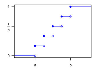
Notation	or
Parameters	; ;
Support
pmf
CDF
Mean
Median
Mode	N/A
Variance
Skewness
Ex. kurtosis
Entropy
MGF
CF

In probability theory and statistics, the discrete uniform distribution is a symmetric probability distribution whereby a finite number of values are equally likely to be observed; every one of n values has equal probability 1/n. Another way of saying "discrete uniform distribution" would be "a known, finite number of outcomes equally likely to happen".

A simple example of the discrete uniform distribution is throwing a fair die. The possible values are 1, 2, 3, 4, 5, 6, and each time the dice is thrown the probability of a given score is 1/6. If two dice are thrown and their values added, the resulting distribution is no longer uniform since not all sums have equal probability.

The discrete uniform distribution itself is inherently non-parametric. It is convenient, however, to represent its values generally by all integers in an interval [a,b], so that a and b become the main parameters of the distribution (often one simply considers the interval [1,n] with the single parameter n). With these conventions, the cumulative distribution function (CDF) of the discrete uniform distribution can be expressed, for any k ∈ [a,b], as

F(k;a,b)={\frac {\lfloor k\rfloor -a+1}{b-a+1}}

Estimation of maximum

This example is described by saying that a sample of k observations is obtained from a uniform distribution on the integers $1,2,\dotsc,N$ , with the problem being to estimate the unknown maximum N. This problem is commonly known as the German tank problem, following the application of maximum estimation to estimates of German tank production during World War II.

The uniformly minimum variance unbiased (UMVU) estimator for the maximum is given by

{\hat {N}}={\frac {k+1}{k}}m-1=m+{\frac {m}{k}}-1

where m is the sample maximum and k is the sample size, sampling without replacement.^[1] This can be seen as a very simple case of maximum spacing estimation.

This has a variance of^[1]

{\frac {1}{k}}{\frac {(N-k)(N+1)}{(k+2)}}\approx {\frac {N^{2}}{k^{2}}}{\text{ for small samples }}k\ll N

so a standard deviation of approximately $\tfrac N k$ , the (population) average size of a gap between samples; compare $\tfrac{m}{k}$ above.

The sample maximum is the maximum likelihood estimator for the population maximum, but, as discussed above, it is biased.

If samples are not numbered but are recognizable or markable, one can instead estimate population size via the capture-recapture method.

Derivation

For any integer m such that k ≤ m ≤ N, the probability that the sample maximum will be equal to m can be computed as follows. The number of different groups of k tanks that can be made from a total of N tanks is given by the binomial coefficient ${\tbinom {N}{k}}$ . Since in this way of counting the permutations of tanks are counted only once, we can order the serial numbers and take note of the maximum of each sample. To compute the probability we have to count the number of ordered samples that can be formed with the last element equal to m and all the other k-1 tanks less or equal to m-1. The number of samples of k-1 tanks that can be made from a total m-1 tanks is given by the binomial coefficient ${\tbinom {m-1}{k-1}}$ , so the probability of having a maximum m is $P(m)={\tbinom {m-1}{k-1}}{\big /}{\tbinom {N}{k}}$ .

Given the total number N and the sample size k, the expected value of the sample maximum is

{\begin{aligned}\mu =\mathrm {E} [m]&=\sum _{m=k}^{N}m{\frac {\tbinom {m-1}{k-1}}{\tbinom {N}{k}}}\\&={\frac {1}{(k-1)!{\tbinom {N}{k}}}}\sum _{m=k}^{N}{\frac {m!}{(m-k)!}}\\&={\frac {k!}{(k-1)!{\tbinom {N}{k}}}}\sum _{m=k}^{N}{\tbinom {m}{k}}\\&=k{\frac {\tbinom {N+1}{k+1}}{\tbinom {N}{k}}}\\&={\frac {k(N+1)}{k+1}},\end{aligned}}

where the hockey-stick identity $\sum _{m=k}^{N}{\tbinom {m}{k}}={\tbinom {N+1}{k+1}}$ was used.

From this equation, the unknown quantity N can be expressed in terms of expectation and sample size as

{\begin{aligned}N&=\mu \left(1+k^{-1}\right)-1.\end{aligned}}

By linearity of the expectation, it is obtained that

{\begin{aligned}\mu \left(1+k^{-1}\right)-1&=\mathrm {E} \left[m\left(1+k^{-1}\right)-1\right],\end{aligned}}

and so an unbiased estimator of N is obtained by replacing the expectation with the observation,

{\begin{aligned}{\hat {N}}&=m\left(1+k^{-1}\right)-1.\end{aligned}}

Besides being unbiased this estimator also attains minimum variance. To show this, first note that the sample maximum is a sufficient statistic for the population maximum since the probability P(m;N) is expressed as a function of m alone. Next it must be shown that the statistics m is also a complete statistic, a special kind of sufficient statistics (demonstration pending). Then the Lehmann–Scheffé theorem implies that ${\hat {N}}$ is the minimum-variance unbiased estimator of N.^[2]

The variance of the estimator is calculated from the variance of the sample maximum

{\begin{aligned}\mathrm {Var} [{\hat {N}}]&={\frac {(k+1)^{2}}{k^{2}}}\mathrm {Var} [m].\end{aligned}}

The variance of the maximum is in turn calculated from the expected values of $m$ and $m^{2}$ . The calculation of the expected value of $m^{2}$ is,

{\begin{aligned}\mathrm {E} [m^{2}]&=\sum _{m=k}^{N}m^{2}{\frac {\tbinom {m-1}{k-1}}{\tbinom {N}{k}}}\\&={\frac {1}{(k-1)!{\tbinom {N}{k}}}}\sum _{m=k}^{N}m{\frac {m!}{(m-k)!}}\\&={\frac {1}{(k-1)!{\tbinom {N}{k}}}}\sum _{m=k}^{N}(m+1-1){\frac {m!}{(m-k)!}}\\&={\frac {1}{(k-1)!{\tbinom {N}{k}}}}\sum _{m=k}^{N}{\frac {(m+1)!}{(m-k)!}}-{\frac {1}{(k-1)!{\tbinom {N}{k}}}}\sum _{m=k}^{N}{\frac {m!}{(m-k)!}}\end{aligned}}

where the second term is the expected value of $m$ . The first term can be expressed in terms of k and N,

{\begin{aligned}{\frac {1}{(k-1)!{\tbinom {N}{k}}}}\sum _{m=k}^{N}{\frac {(m+1)!}{(m-k)!}}&={\frac {(k+1)!}{(k-1)!{\tbinom {N}{k}}}}\sum _{m=k}^{N}{\tbinom {m+1}{k+1}}\\&={\frac {k(k+1)}{\tbinom {N}{k}}}\sum _{n=k+1}^{N+1}{\tbinom {n}{k+1}}\\&={\frac {k(k+1)}{\tbinom {N}{k}}}{\tbinom {N+2}{k+2}}\\&={\frac {k(N+2)(N+1)}{(k+2)}}\end{aligned}}

where the replacement $n=m+1$ was made and the hockey-stick identity used. Replacing this result and the expectation of $m$ in the equation of $E[m^{2}]$ ,

{\begin{aligned}\mathrm {E} [m^{2}]&={\frac {k(N+2)(N+1)}{(k+2)}}-{\frac {k(N+1)}{k+1}}\\&=k(N+1){\Big (}{\frac {N+2}{k+2}}-{\frac {1}{k+1}}{\Big )}\\&={\frac {k(N+1)(kN+k+N)}{(k+1)(k+2)}}\end{aligned}}

The variance of $m$ is then obtained,

{\begin{aligned}\mathrm {Var} [m]&=\mathrm {E} [m^{2}]-\mathrm {E} [m]^{2}\\&={\frac {k(N+1)}{(k+1)}}{\Big (}{\frac {kN+k+N}{k+2}}-{\frac {k(N+1)}{k+1}}{\Big )}\\&={\frac {k(N+1)}{(k+1)}}{\frac {(N-k)}{(k+2)(k+1)}}\\&={\frac {k(N+1)(N-k)}{(k+1)^{2}(k+2)}}\end{aligned}}

Finally the variance of the estimator ${\hat {N}}$ can be calculated,

{\begin{aligned}\mathrm {Var} [{\hat {N}}]&={\frac {(k+1)^{2}}{k^{2}}}\mathrm {Var} [m]\\&={\frac {(k+1)^{2}}{k^{2}}}{\frac {k(N+1)(N-k)}{(k+1)^{2}(k+2)}}\\&={\frac {(N+1)(N-k)}{k(k+2)}}.\end{aligned}}

Random permutation

See rencontres numbers for an account of the probability distribution of the number of fixed points of a uniformly distributed random permutation.

Notes

References

1 2 Johnson, Roger (1994), "Estimating the Size of a Population", Teaching Statistics, 16 (2 (Summer)), doi:10.1111/j.1467-9639.1994.tb00688.x
↑ G. A. Young and R. L Smith (2005) Essentials of Statistical Inference, Cambridge University Press, Cambridge, UK, p. 95

This article is issued from Wikipedia. The text is licensed under Creative Commons - Attribution - Sharealike. Additional terms may apply for the media files.

[Johnson-1] 1 2 Johnson, Roger (1994), "Estimating the Size of a Population", Teaching Statistics, 16 (2 (Summer)), doi:10.1111/j.1467-9639.1994.tb00688.x

[2] G. A. Young and R. L Smith (2005) Essentials of Statistical Inference, Cambridge University Press, Cambridge, UK, p. 95

Probability distributions
List
Discrete univariate with finite support	Benford Bernoulli beta-binomial binomial categorical hypergeometric Poisson binomial Rademacher discrete uniform Zipf Zipf–Mandelbrot
Discrete univariate with infinite support	beta negative binomial Borel Conway–Maxwell–Poisson discrete phase-type Delaporte extended negative binomial Gauss–Kuzmin geometric logarithmic negative binomial parabolic fractal Poisson Skellam Yule–Simon zeta
Continuous univariate supported on a bounded interval	arcsine ARGUS Balding–Nichols Bates beta beta rectangular Irwin–Hall Kumaraswamy logit-normal noncentral beta raised cosine reciprocal triangular U-quadratic uniform Wigner semicircle
Continuous univariate supported on a semi-infinite interval	Benini Benktander 1st kind Benktander 2nd kind beta prime Burr chi-squared chi Dagum Davis exponential-logarithmic Erlang exponential F folded normal Flory–Schulz Fréchet gamma gamma/Gompertz generalized inverse Gaussian Gompertz half-logistic half-normal Hotelling's T-squared hyper-Erlang hyperexponential hypoexponential inverse chi-squared scaled inverse chi-squared inverse Gaussian inverse gamma Kolmogorov Lévy log-Cauchy log-Laplace log-logistic log-normal Lomax matrix-exponential Maxwell–Boltzmann Maxwell–Jüttner Mittag-Leffler Nakagami noncentral chi-squared Pareto phase-type poly-Weibull Rayleigh relativistic Breit–Wigner Rice shifted Gompertz truncated normal type-2 Gumbel Weibull Discrete Weibull Wilks's lambda
Continuous univariate supported on the whole real line	Cauchy exponential power Fisher's z Gaussian q generalized normal generalized hyperbolic geometric stable Gumbel Holtsmark hyperbolic secant Johnson's S_U Landau Laplace asymmetric Laplace logistic noncentral t normal (Gaussian) normal-inverse Gaussian skew normal slash stable Student's t type-1 Gumbel Tracy–Widom variance-gamma Voigt
Continuous univariate with support whose type varies	generalized extreme value generalized Pareto Marchenko–Pastur q-exponential q-Gaussian q-Weibull shifted log-logistic Tukey lambda
Mixed continuous-discrete univariate	rectified Gaussian
Multivariate (joint)	Discrete Ewens multinomial Dirichlet-multinomial negative multinomial Continuous Dirichlet generalized Dirichlet multivariate Laplace multivariate normal multivariate stable multivariate t normal-inverse-gamma normal-gamma Matrix-valued inverse matrix gamma inverse-Wishart matrix normal matrix t matrix gamma normal-inverse-Wishart normal-Wishart Wishart
Directional	Univariate (circular) directional Circular uniform univariate von Mises wrapped normal wrapped Cauchy wrapped exponential wrapped asymmetric Laplace wrapped Lévy Bivariate (spherical) Kent Bivariate (toroidal) bivariate von Mises Multivariate von Mises–Fisher Bingham
Degenerate and singular	Degenerate Dirac delta function Singular Cantor
Families	Circular compound Poisson elliptical exponential natural exponential location–scale maximum entropy mixture Pearson Tweedie wrapped

Probability mass function n = 5 where n = b − a + 1
Cumulative distribution function
Notation	${\mathcal {U}}\{a,b\}$ or ${\mathrm {unif}}\{a,b\}$
Parameters	$a \in \{\dots,-2,-1,0,1,2,\dots\}\,$ $b \in \{\dots,-2,-1,0,1,2,\dots\}, b \ge a$ $n=b-a+1\,$
Support	$k\in \{a,a+1,\dots ,b-1,b\}\,$
pmf	${\frac {1}{n}}$
CDF	${\frac {\lfloor k\rfloor -a+1}{n}}$
Mean	${\frac {a+b}{2}}\,$
Median	${\frac {a+b}{2}}\,$
Mode	N/A
Variance	${\frac {(b-a+1)^{2}-1}{12}}$
Skewness	$0\,$
Ex. kurtosis	$-{\frac {6(n^{2}+1)}{5(n^{2}-1)}}\,$
Entropy	$\ln(n)\,$
MGF	${\frac {e^{{at}}-e^{{(b+1)t}}}{n(1-e^{t})}}\,$
CF	${\frac {e^{{iat}}-e^{{i(b+1)t}}}{n(1-e^{{it}})}}$