Tukey lambda distribution

Tukey lambda distribution
	Probability density function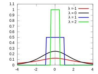
Notation	Tukey(λ)
Parameters	λ ∈ R — shape parameter
Support	x ∈ [−1/λ, 1/λ] for λ > 0,; x ∈ R for λ ≤ 0
PDF
CDF
Mean
Median	0
Mode	0
Variance	;
Skewness
Ex. kurtosis	; ;
Entropy	[1]
CF	[2]

Formalized by John Tukey, the Tukey lambda distribution is a continuous, symmetric probability distribution defined in terms of its quantile function. It is typically used to identify an appropriate distribution (see the comments below) and not used in statistical models directly.

The Tukey lambda distribution has a single shape parameter, λ, and as with other probability distributions, it can be transformed with a location parameter, μ, and a scale parameter, σ. Since the general form of probability distribution can be expressed in terms of the standard distribution, the subsequent formulas are given for the standard form of the function.

Quantile function

For the standard form of the Tukey lambda distribution, the quantile function, $Q(p)$ , (i.e. the inverse of the cumulative distribution function) and the quantile density function ( $q=dQ/dp$ ) are

Q\left(p;\lambda\right) = \begin{cases} \frac{ 1 }{ \lambda } \left[p^\lambda - (1 - p)^\lambda\right], & \mbox{if } \lambda \ne 0 \\ \log(\frac{p}{1-p}), & \mbox{if } \lambda = 0, \end{cases}

q\left(p;\lambda \right)=p^{(\lambda -1)}+\left(1-p\right)^{(\lambda -1)}.

For most values of the shape parameter, λ, the probability density function (PDF) and cumulative distribution function (CDF) must be computed numerically. The Tukey lambda distribution has a simple, closed form for the CDF and/or PDF only for a few exceptional values of the shape parameter, for example: λ = 2, 1, ½, 0 (see uniform distribution and the logistic distribution).

However, for any value of λ both the CDF and PDF can be tabulated for any number of cumulative probabilities, p, using the quantile function Q to calculate the value x, for each cumulative probability p, with the probability density given by ¹⁄_q, the reciprocal of the quantile density function. As is the usual case with statistical distributions, the Tukey lambda distribution can readily be used by looking up values in a prepared table.

Moments

The Tukey lambda distribution is symmetric around zero, therefore the expected value of this distribution is equal to zero. The variance exists for λ > −½ and is given by the formula (except when λ = 0)

\operatorname{Var}[X] = \frac{2}{\lambda^2}\bigg(\frac{1}{1+2\lambda} - \frac{\Gamma(\lambda+1)^2}{\Gamma(2\lambda+2)}\bigg).

More generally, the n-th order moment is finite when λ > −1/n and is expressed in terms of the beta function Β(x,y) (except when λ = 0) :

\mu_n = \operatorname{E}[X^n] = \frac{1}{\lambda^n} \sum_{k=0}^n (-1)^k {n \choose k}\, \Beta(\lambda k+1,\, \lambda(n-k)+1 ).

Note that due to symmetry of the density function, all moments of odd orders are equal to zero.

L-moments

Differently from the central moments, L-moments can be expressed in a closed form. The L-moment of order r>1 is given by^[3]

L_{r} \lambda=\sum_{k=0}^{r-1} (-1)^{r-k-1} \binom{r-1}{k} \binom{r+k-1}{k} \left(\frac{1}{k+1+\lambda}+\frac{(-1)^{r}}{k+1+\lambda} \right).

The first six L-moments can be presented as follows:^[3]

L_{1}=0

L_2 \lambda = - \frac{2}{1 + \lambda} + \frac{4}{2 + \lambda}

L_3 =0

L_4 \lambda = - \frac{2}{1+\lambda} + \frac{24}{2+\lambda} - \frac{60}{3+\lambda} + \frac{60}{4+\lambda}

L_5 =0

L_6 \lambda = -\frac{2}{1+\lambda} + \frac{60}{2+\lambda} - \frac{420}{3+\lambda} +\frac{1120}{4+\lambda}-\frac{1260}{5+\lambda}+\frac{504}{6+\lambda}.

Comments

The Tukey lambda distribution is actually a family of distributions that can approximate a number of common distributions. For example,

λ = −1	approx. Cauchy C(0,π)
λ = 0	exactly logistic
λ = 0.14	approx. normal N(0, 2.142)
λ = 0.5	strictly concave ( $\cap$ -shaped)
λ = 1	exactly uniform U(−1, 1)
λ = 2	exactly uniform U(−½, ½)

The most common use of this distribution is to generate a Tukey lambda PPCC plot of a data set. Based on the PPCC plot, an appropriate model for the data is suggested. For example, if the maximum correlation occurs for a value of λ at or near 0.14, then the data can be modeled with a normal distribution. Values of λ less than this imply a heavy-tailed distribution (with −1 approximating a Cauchy). That is, as the optimal value of lambda goes from 0.14 to −1, increasingly heavy tails are implied. Similarly, as the optimal value of λ becomes greater than 0.14, shorter tails are implied.

Since the Tukey lambda distribution is a symmetric distribution, the use of the Tukey lambda PPCC plot to determine a reasonable distribution to model the data only applies to symmetric distributions. A histogram of the data should provide evidence as to whether the data can be reasonably modeled with a symmetric distribution.^[4]

References

↑ Vasicek, Oldrich (1976), "A Test for Normality Based on Sample Entropy", Journal of the Royal Statistical Society, Series B, 38 (1): 54–59.
↑ Shaw, W. T.; McCabe, J. (2009), "Monte Carlo sampling given a Characteristic Function: Quantile Mechanics in Momentum Space", arXiv:0903.1592
1 2 Karvanen, Juha; Nuutinen, Arto (2008). "Characterizing the generalized lambda distribution by L-moments". Computational Statistics & Data Analysis. 52: 1971–1983. arXiv:math/0701405. doi:10.1016/j.csda.2007.06.021.
↑ Joiner, Brian L.; Rosenblatt, Joan R. (1971), "Some Properties of the Range in Samples from Tukey's Symmetric Lambda Distributions", Journal of the American Statistical Association, 66 (334): 394–399, doi:10.2307/2283943, JSTOR 2283943

External links

Tukey-Lambda Distribution

This article incorporates public domain material from the National Institute of Standards and Technology website http://www.nist.gov.

This article is issued from Wikipedia. The text is licensed under Creative Commons - Attribution - Sharealike. Additional terms may apply for the media files.

[1] Vasicek, Oldrich (1976), "A Test for Normality Based on Sample Entropy", Journal of the Royal Statistical Society, Series B, 38 (1): 54–59.

[2] Shaw, W. T.; McCabe, J. (2009), "Monte Carlo sampling given a Characteristic Function: Quantile Mechanics in Momentum Space", arXiv:0903.1592

[kar:08-3] 1 2 Karvanen, Juha; Nuutinen, Arto (2008). "Characterizing the generalized lambda distribution by L-moments". Computational Statistics & Data Analysis. 52: 1971–1983. arXiv:math/0701405. doi:10.1016/j.csda.2007.06.021.

[4] Joiner, Brian L.; Rosenblatt, Joan R. (1971), "Some Properties of the Range in Samples from Tukey's Symmetric Lambda Distributions", Journal of the American Statistical Association, 66 (334): 394–399, doi:10.2307/2283943, JSTOR 2283943

Probability distributions
List
Discrete univariate with finite support	Benford Bernoulli beta-binomial binomial categorical hypergeometric Poisson binomial Rademacher discrete uniform Zipf Zipf–Mandelbrot
Discrete univariate with infinite support	beta negative binomial Borel Conway–Maxwell–Poisson discrete phase-type Delaporte extended negative binomial Gauss–Kuzmin geometric logarithmic negative binomial parabolic fractal Poisson Skellam Yule–Simon zeta
Continuous univariate supported on a bounded interval	arcsine ARGUS Balding–Nichols Bates beta beta rectangular Irwin–Hall Kumaraswamy logit-normal noncentral beta raised cosine reciprocal triangular U-quadratic uniform Wigner semicircle
Continuous univariate supported on a semi-infinite interval	Benini Benktander 1st kind Benktander 2nd kind beta prime Burr chi-squared chi Dagum Davis exponential-logarithmic Erlang exponential F folded normal Flory–Schulz Fréchet gamma gamma/Gompertz generalized inverse Gaussian Gompertz half-logistic half-normal Hotelling's T-squared hyper-Erlang hyperexponential hypoexponential inverse chi-squared scaled inverse chi-squared inverse Gaussian inverse gamma Kolmogorov Lévy log-Cauchy log-Laplace log-logistic log-normal Lomax matrix-exponential Maxwell–Boltzmann Maxwell–Jüttner Mittag-Leffler Nakagami noncentral chi-squared Pareto phase-type poly-Weibull Rayleigh relativistic Breit–Wigner Rice shifted Gompertz truncated normal type-2 Gumbel Weibull Discrete Weibull Wilks's lambda
Continuous univariate supported on the whole real line	Cauchy exponential power Fisher's z Gaussian q generalized normal generalized hyperbolic geometric stable Gumbel Holtsmark hyperbolic secant Johnson's S_U Landau Laplace asymmetric Laplace logistic noncentral t normal (Gaussian) normal-inverse Gaussian skew normal slash stable Student's t type-1 Gumbel Tracy–Widom variance-gamma Voigt
Continuous univariate with support whose type varies	generalized extreme value generalized Pareto Marchenko–Pastur q-exponential q-Gaussian q-Weibull shifted log-logistic Tukey lambda
Mixed continuous-discrete univariate	rectified Gaussian
Multivariate (joint)	Discrete Ewens multinomial Dirichlet-multinomial negative multinomial Continuous Dirichlet generalized Dirichlet multivariate Laplace multivariate normal multivariate stable multivariate t normal-inverse-gamma normal-gamma Matrix-valued inverse matrix gamma inverse-Wishart matrix normal matrix t matrix gamma normal-inverse-Wishart normal-Wishart Wishart
Directional	Univariate (circular) directional Circular uniform univariate von Mises wrapped normal wrapped Cauchy wrapped exponential wrapped asymmetric Laplace wrapped Lévy Bivariate (spherical) Kent Bivariate (toroidal) bivariate von Mises Multivariate von Mises–Fisher Bingham
Degenerate and singular	Degenerate Dirac delta function Singular Cantor
Families	Circular compound Poisson elliptical exponential natural exponential location–scale maximum entropy mixture Pearson Tweedie wrapped

Tukey lambda distribution
Probability density function
Notation	Tukey(λ)
Parameters	λ ∈ R — shape parameter
Support	x ∈ [−1/λ, 1/λ] for λ > 0, x ∈ R for λ ≤ 0
PDF	$(Q(p;\lambda ),q(p;\lambda )^{-1}),\,0\leq \,p\,\leq \,1$
CDF	$(e^{-x}+1)^{-1},\,\,\lambda\,=\,0$
Mean	$0,\,\,\lambda > -1$
Median	0
Mode	0
Variance	$\frac{2}{\lambda^2}\bigg(\frac{1}{1+2\lambda}-\frac{\Gamma(\lambda+1)^2}{\Gamma(2\lambda+2)}\bigg),\,\,\lambda > -1/2$ $\frac{ \pi^{2} }{ 3 },\,\,\lambda\,=\,0$
Skewness	$0,\,\,\lambda > -1/3$
Ex. kurtosis	${\frac {(2\lambda +1)^{2}}{2(4\lambda +1)}}\,{\frac {g_{2}^{2}{\big (}3g_{2}^{2}-4g_{1}g_{3}+g_{4}{\big )}}{g_{4}{\big (}g_{1}^{2}-g_{2}{\big )}^{2}}}\,-\,3,$ $1.2,\,\,\lambda \,=\,0,$ ${\text{where}}\,g_{k}\,=\,\Gamma (k\lambda +1)\,{\text{and}}\,\lambda \,>\,-1/4.$
Entropy	$h(\lambda )=\int _{0}^{1}\log(q(p;\lambda ))\,dp$ ^[1]
CF	$\phi(t;\lambda) = \int_0^1 \exp (\,i t\,Q(p;\lambda))\,dp$ ^[2]