Median

Finding the median in sets of data with an odd and even number of values

The median is the value separating the higher half from the lower half of a data sample (a population or a probability distribution). For a data set, it may be thought of as the "middle" value. For example, in the data set {1, 3, 3, 6, 7, 8, 9}, the median is 6, the fourth largest, and also the fourth smallest, number in the sample. For a continuous probability distribution, the median is the value such that a number is equally likely to fall above or below it.

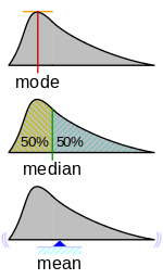
The median is a commonly used measure of the properties of a data set in statistics and probability theory. The basic advantage of the median in describing data compared to the mean (often simply described as the "average") is that it is not skewed so much by extremely large or small values, and so it may give a better idea of a "typical" value. For example, in understanding statistics like household income or assets which vary greatly, a mean may be skewed by a small number of extremely high or low values. Median income, for example, may be a better way to suggest what a "typical" income is.

Because of this, the median is of central importance in robust statistics, as it is the most resistant statistic, having a breakdown point of 50%: so long as no more than half the data are contaminated, the median will not give an arbitrarily large or small result.

Finite set of numbers

The median of a finite list of numbers can be found by arranging all the numbers from smallest to greatest.

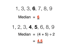
If there is an odd number of numbers, the middle one is picked. For example, consider the list of numbers

1, 3, 3, 6, 7, 8, 9

This list contains seven numbers. The median is the fourth of them, which is 6.

If there is an even number of observations, then there is no single middle value; the median is then usually defined to be the mean of the two middle values.^[1]^[2] For example, in the data set

1, 2, 3, 4, 5, 6, 8, 9

the median is the mean of the middle two numbers: this is $(4+5)/2$ , which is $4.5$ . (In more technical terms, this interprets the median as the fully trimmed mid-range).

The formula used to find the index of the middle number of a data set of n numerically ordered numbers is $(n+1)/2$ . This either gives the middle number (for an odd number of values) or the halfway point between the two middle values. For example, with 14 values, the formula will give an index of 7.5, and the median will be taken by averaging the seventh (the floor of this index) and eighth (the ceiling of this index) values. So the median can be represented by the following formula:

\mathrm {median} (a)={\frac {a_{\lceil \#x\div 2\rceil }+a_{\lceil \#x\div 2+1\rceil }}{2}}

Comparison of common averages of values { 1, 2, 2, 3, 4, 7, 9 }
Type	Description	Example	Result
Arithmetic mean	Sum of values of a data set divided by number of values: $\scriptstyle {\bar {x}}={\frac {1}{n}}\sum _{{i=1}}^{n}x_{i}$	(1+2+2+3+4+7+9) / 7	4
Median	Middle value separating the greater and lesser halves of a data set	1, 2, 2, 3, 4, 7, 9	3
Mode	Most frequent value in a data set	1, 2, 2, 3, 4, 7, 9	2

One can find the median using the Stem-and-Leaf Plot.

There is no widely accepted standard notation for the median, but some authors represent the median of a variable x either as x͂ or as μ_1/2^[1] sometimes also M.^[3]^[4] In any of these cases, the use of these or other symbols for the median needs to be explicitly defined when they are introduced.

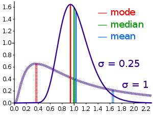
The median is used primarily for skewed distributions, which it summarizes differently from the arithmetic mean. Consider the multiset { 1, 2, 2, 2, 3, 14 }. The median is 2 in this case, (as is the mode), and it might be seen as a better indication of central tendency (less susceptible to the exceptionally large value in data) than the arithmetic mean of 4.

The median is a popular summary statistic used in descriptive statistics, since it is simple to understand and easy to calculate, while also giving a measure that is more robust in the presence of outlier values than is the mean. The widely cited empirical relationship between the relative locations of the mean and the median for skewed distributions is, however, not generally true.^[5] There are, however, various relationships for the absolute difference between them; see below.

With an even number of observations (as shown above) no value need be exactly at the value of the median. Nonetheless, the value of the median is uniquely determined with the usual definition. A related concept, in which the outcome is forced to correspond to a member of the sample, is the medoid.

In a population, at most half have values strictly less than the median and at most half have values strictly greater than it. If each group contains less than half the population, then some of the population is exactly equal to the median. For example, if a < b < c, then the median of the list {a, b, c} is b, and, if a < b < c < d, then the median of the list {a, b, c, d} is the mean of b and c; i.e., it is (b + c)/2. Indeed, as it is based on the middle data in a group, it is not necessary to even know the value of extreme results in order to calculate a median. For example, in a psychology test investigating the time needed to solve a problem, if a small number of people failed to solve the problem at all in the given time a median can still be calculated.^[6]

The median can be used as a measure of location when a distribution is skewed, when end-values are not known, or when one requires reduced importance to be attached to outliers, e.g., because they may be measurement errors.

A median is only defined on ordered one-dimensional data, and is independent of any distance metric. A geometric median, on the other hand, is defined in any number of dimensions.

The median is one of a number of ways of summarising the typical values associated with members of a statistical population; thus, it is a possible location parameter. The median is the 2nd quartile, 5th decile, and 50th percentile. Since the median is the same as the second quartile, its calculation is illustrated in the article on quartiles. A median can be worked out for ranked but not numerical classes (e.g. working out a median grade when students are graded from A to F), although the result might be halfway between grades if there is an even number of cases.

When the median is used as a location parameter in descriptive statistics, there are several choices for a measure of variability: the range, the interquartile range, the mean absolute deviation, and the median absolute deviation.

For practical purposes, different measures of location and dispersion are often compared on the basis of how well the corresponding population values can be estimated from a sample of data. The median, estimated using the sample median, has good properties in this regard. While it is not usually optimal if a given population distribution is assumed, its properties are always reasonably good. For example, a comparison of the efficiency of candidate estimators shows that the sample mean is more statistically efficient than the sample median when data are uncontaminated by data from heavy-tailed distributions or from mixtures of distributions, but less efficient otherwise, and that the efficiency of the sample median is higher than that for a wide range of distributions. More specifically, the median has a 64% efficiency compared to the minimum-variance mean (for large normal samples), which is to say the variance of the median will be ~50% greater than the variance of the mean—see asymptotic efficiency and references therein.

Probability distributions

Geometric visualisation of the mode, median and mean of an arbitrary probability density function.^[7]

For any probability distribution on the real line R with cumulative distribution function F, regardless of whether it is any kind of continuous probability distribution, in particular an absolutely continuous distribution (which has a probability density function), or a discrete probability distribution, a median is by definition any real number m that satisfies the inequalities

\operatorname {P} (X\leq m)\geq {\frac {1}{2}}{\text{ and }}\operatorname {P} (X\geq m)\geq {\frac {1}{2}}\,\!

or, equivalently, the inequalities

\int _{(-\infty ,m]}dF(x)\geq {\frac {1}{2}}{\text{ and }}\int _{[m,\infty )}dF(x)\geq {\frac {1}{2}}\,\!

in which a Lebesgue–Stieltjes integral is used. For an absolutely continuous probability distribution with probability density function ƒ, the median satisfies

\operatorname {P} (X\leq m)=\operatorname {P} (X\geq m)=\int _{-\infty }^{m}f(x)\,dx={\frac {1}{2}}.\,\!

Any probability distribution on R has at least one median, but in specific cases there may be more than one median. Specifically, if a probability distribution is zero on an interval [a, b], and the cumulative distribution function at a is 1/2, any value between a and b will also be a median.

Medians of particular distributions

The medians of certain types of distributions can be easily calculated from their parameters; furthermore, they exist even for some distributions lacking a well-defined mean, such as the Cauchy distribution:

The median of a symmetric unimodal distribution coincides with the mode.
The median of a symmetric distribution which possesses a mean μ also takes the value μ.
- The median of a normal distribution with mean μ and variance σ² is μ. In fact, for a normal distribution, mean = median = mode.
- The median of a uniform distribution in the interval [a, b] is (a + b) / 2, which is also the mean.
The median of a Cauchy distribution with location parameter x₀ and scale parameter y is x₀, the location parameter.
The median of a power law distribution x^−a, with exponent a > 1 is 2^{1/(a − 1)}x_min, where x_min is the minimum value for which the power law holds^[8]
The median of an exponential distribution with rate parameter λ is the natural logarithm of 2 divided by the rate parameter: λ⁻¹ln 2.
The median of a Weibull distribution with shape parameter k and scale parameter λ is λ(ln 2)^1/k.

Populations

Optimality property

The mean absolute error of a real variable c with respect to the random variable X is

E(\left|X-c\right|)\,

Provided that the probability distribution of X is such that the above expectation exists, then m is a median of X if and only if m is a minimizer of the mean absolute error with respect to X.^[9] In particular, m is a sample median if and only if m minimizes the arithmetic mean of the absolute deviations.

More generally, a median is defined as a minimum of

E(|X-c|-|X|),

as discussed below in the section on multivariate medians (specifically, the spatial median).

This optimization-based definition of the median is useful in statistical data-analysis, for example, in k-medians clustering.

Unimodal distributions

Comparison of mean, median and mode of two log-normal distributions with different skewness.

It can be shown for a unimodal distribution that the median ${\tilde {X}}$ and the mean ${\bar {X}}$ lie within (3/5)^1/2 ≈ 0.7746 standard deviations of each other.^[10] In symbols,

{\frac {\left|{\tilde {X}}-{\bar {X}}\right|}{\sigma }}\leq \left({\frac {3}{5}}\right)^{\frac {1}{2}}

where |·| is the absolute value.

A similar relation holds between the median and the mode: they lie within 3^1/2 ≈ 1.732 standard deviations of each other:

{\frac {|{\tilde {X}}-\mathrm {mode} |}{\sigma }}\leq 3^{\frac {1}{2}}.

Inequality relating means and medians

If the distribution has finite variance, then the distance between the median and the mean is bounded by one standard deviation.

This bound was proved by Mallows,^[11] who used Jensen's inequality twice, as follows. We have

{\begin{aligned}|\mu -m|=|\operatorname {E} (X-m)|&\leq \operatorname {E} (|X-m|)\\&\leq \operatorname {E} (|X-\mu |)\\&\leq {\sqrt {\operatorname {E} \left((X-\mu )^{2}\right)}}=\sigma .\end{aligned}}

The first and third inequalities come from Jensen's inequality applied to the absolute-value function and the square function, which are each convex. The second inequality comes from the fact that a median minimizes the absolute deviation function

a\mapsto \operatorname {E} (|X-a|).\,

This proof also follows directly from Cantelli's inequality.^[12] The result can be generalized to obtain a multivariate version of the inequality,^[13] as follows:

{\begin{aligned}\|\mu -m\|=\|\operatorname {E} (X-m)\|&\leq \operatorname {E} \|X-m\|\\&\leq \operatorname {E} (\|X-\mu \|)\\&\leq {\sqrt {\operatorname {E} \left(\|X-\mu \|^{2}\right)}}={\sqrt {\operatorname {trace} \left(\operatorname {var} (X)\right)}}\end{aligned}}

where m is a spatial median, that is, a minimizer of the function $a\mapsto \operatorname {E} (\|X-a\|).\,$ The spatial median is unique when the data-set's dimension is two or more.^[14]^[15] An alternative proof uses the one-sided Chebyshev inequality; it appears in an inequality on location and scale parameters.

Jensen's inequality for medians

Jensen's inequality states that for any random variable x with a finite expectation E(x) and for any convex function f

f[E(x)]\leq E[f(x)]

It has been shown^[16] that if x is a real variable with a unique median m and f is a C function then

f(m)\leq \operatorname {Median} [f(x)]

A C function is a real valued function, defined on the set of real numbers R, with the property that for any real t

f^{-1}\left(\,(-\infty ,t]\,\right)=\{x\in R\mid f(x)\leq t\}

is a closed interval, a singleton or an empty set.

Medians for samples

The sample median

Efficient computation of the sample median

Even though comparison-sorting n items requires $Ω (n log n)$ operations, selection algorithms can compute the $k$ 'th-smallest of $n$ items with only $Θ(n)$ operations. This includes the median, which is the $n / 2$ 'th order statistic (or for an even number of samples, the arithmetic mean of the two middle order statistics).

Selection algorithms still have the downside of requiring $Ω(n)$ memory, that is, they need to have the full sample (or a linear-sized portion of it) in memory. Because this, as well as the linear time requirement, can be prohibitive, several estimation procedures for the median have been developed. A simple one is the median of three rule, which estimates the median as the median of a three-element subsample; this is commonly used as a subroutine in the quicksort sorting algorithm, which uses an estimate of its input's median. A more robust estimator is Tukey's ninther, which is the median of three rule applied with limited recursion:^[17] if $A$ is the sample laid out as an array, and

med3(A) = median(A [1], A [n / 2], A [n])

,

then

ninther(A) = med3(med3(A [1 ... 1 / 3 n]), med3(A [1 / 3 n ... 2 / 3 n]), med3(A [2 / 3 n ... n]))

The remedian is an estimator for the median that requires linear time but sub-linear memory, operating in a single pass over the sample.^[18]

Easy explanation of the sample median

In individual series (if number of observation is very low) first one must arrange all the observations in order. Then count(n) is the total number of observation in given data.

If n is odd then Median (M) = value of ((n + 1)/2)th item term.

If n is even then Median (M) = value of [(n/2)th item term + (n/2 + 1)th item term]/2

For an odd number of values

As an example, we will calculate the sample median for the following set of observations: 1, 5, 2, 8, 7.

Start by sorting the values: 1, 2, 5, 7, 8.

In this case, the median is 5 since it is the middle observation in the ordered list.

The median is the ((n + 1)/2)th item, where n is the number of values. For example, for the list {1, 2, 5, 7, 8}, we have n = 5, so the median is the ((5 + 1)/2)th item.

median = (6/2)th item

median = 3rd item

median = 5

For an even number of values

As an example, we will calculate the sample median for the following set of observations: 1, 6, 2, 8, 7, 2.

Start by sorting the values: 1, 2, 2, 6, 7, 8.

In this case, the arithmetic mean of the two middlemost terms is (2 + 6)/2 = 4. Therefore, the median is 4 since it is the arithmetic mean of the middle observations in the ordered list.

Sampling distribution

The distributions of both the sample mean and the sample median were determined by Laplace.^[19] The distribution of the sample median from a population with a density function $f(x)$ is asymptotically normal with mean $m$ and variance^[20]

{\frac {1}{4nf(m)^{2}}}

where $m$ is the median of $f(x)$ and $n$ is the sample size.

These results have also been extended.^[21] It is now known for the $p$ -th quantile that the distribution of the sample $p$ -th quantile is asymptotically normal around the $p$ -th quantile with variance equal to

{\frac {p(1-p)}{nf(x_{p})^{2}}}

where $f(x_{p})$ is the value of the distribution density at the $p$ -th quantile.

In the case of a discrete variable, the sampling distribution of the median for small-samples can be investigated as follows. We take the sample size to be an odd number $N=2n+1$ . If a given value $v$ is to be the median of the sample then two conditions must be satisfied. The first is that at most $n$ observations can have a value of $v-1$ or less. The second is that at most $n$ observations can have a value of $v+1$ or more. Let $i$ be the number of observations which have a value of $v-1$ or less and let $k$ be the number of observations which have a value of $v+1$ or more. Then $i$ and $k$ both have a minimum value of 0 and a maximum of $n$ . If an observation has a value below $v$ , it is not relevant how far below $v$ it is and conversely, if an observation has a value above $v$ , it is not relevant how far above $v$ it is. We can therefore represent the observations as following a trinomial distribution with probabilities $F(v-1)$ , $f(v)$ and $1-F(v)$ . The probability that the median $m$ will have a value $v$ is then given by

\Pr(m=v)=\sum _{i=0}^{n}\sum _{k=0}^{n}{\frac {N!}{i!(N-i-k)!k!}}[F(v-1)]^{i}[f(v)]^{N-i-k}[1-F(v)]^{k}.

Summing this over all values of $v$ defines a proper distribution and gives a unit sum. In practice, the function $f(v)$ will often not be known but it can be estimated from an observed frequency distribution. An example is given in the following table where the actual distribution is not known but a sample of 3,800 observations allows a sufficiently accurate assessment of $f(v)$ .

v	0	0.5	1	1.5	2	2.5	3	3.5	4	4.5	5
f(v)	0.000	0.008	0.010	0.013	0.083	0.108	0.328	0.220	0.202	0.023	0.005
F(v)	0.000	0.008	0.018	0.031	0.114	0.222	0.550	0.770	0.972	0.995	1.000

Using these data it is possible to investigate the effect of sample size on the standard errors of the mean and median. The observed mean is 3.16, the observed raw median is 3 and the observed interpolated median is 3.174. The following table gives some comparison statistics. The standard error of the median is given both from the above expression for $pr(m=v)$ and from the asymptotic approximation given earlier.

Sample size Statistic	3	9	15	21
Expected value of median	3.198	3.191	3.174	3.161
Standard error of median (above formula)	0.482	0.305	0.257	0.239
Standard error of median (asymptotic approximation)	0.879	0.508	0.393	0.332
Standard error of mean	0.421	0.243	0.188	0.159

The expected value of the median falls slightly as sample size increases while, as would be expected, the standard errors of both the median and the mean are proportionate to the inverse square root of the sample size. The asymptotic approximation errs on the side of caution by overestimating the standard error.

In the case of a continuous variable, the following argument can be used. If a given value $v$ is to be the median, then one observation must take the value $v$ . The elemental probability of this is $f(v)\,dv$ . Then, of the remaining $2n$ observations, exactly $n$ of them must be above $v$ and the remaining $n$ below. The probability of this is the $n$ th term of a binomial distribution with parameters $F(v)$ and $2n$ . Finally we multiply by $2n+1$ since any of the observations in the sample can be the median observation. Hence the elemental probability of the median at the point $v$ is given by

f(v){\frac {(2n)!}{n!n!}}[F(v)]^{n}[1-F(v)]^{n}(2n+1)\,dv.

Now we introduce the beta function. For integer arguments $\alpha$ and $\beta$ , this can be expressed as $\mathrm {B} (\alpha ,\beta )=(\alpha -1)!(\beta -1)!/(\alpha +\beta -1)!$ . Also, we note that $f(v)=dF(v)/dv$ . Using these relationships and setting both $\alpha$ and $\beta$ equal to $(n+1)$ allows the last expression to be written as

{\frac {[F(v)]^{n}[1-F(v)]^{n}}{\mathrm {B} (n+1,n+1)}}\,dF(v)

Hence the density function of the median is a symmetric beta distribution over the unit interval which supports $F(v)$ . Its mean, as we would expect, is 0.5 and its variance is $1/(4(N+2))$ . The corresponding variance of the sample median is

{\frac {1}{4(N+2)f(m)^{2}}}.

However this finding can only be used if the density function $f(v)$ is known or can be assumed. As this will not always be the case, the median variance has to be estimated sometimes from the sample data.

Estimation of variance from sample data

The value of $(2f(x))^{-2}$ —the asymptotic value of $n^{-{\frac {1}{2}}}(\nu -m)$ where $\nu$ is the population median—has been studied by several authors. The standard "delete one" jackknife method produces inconsistent results.^[22] An alternative—the "delete k" method—where $k$ grows with the sample size has been shown to be asymptotically consistent.^[23] This method may be computationally expensive for large data sets. A bootstrap estimate is known to be consistent,^[24] but converges very slowly (order of $n^{-{\frac {1}{4}}}$ ).^[25] Other methods have been proposed but their behavior may differ between large and small samples.^[26]

Efficiency

The efficiency of the sample median, measured as the ratio of the variance of the mean to the variance of the median, depends on the sample size and on the underlying population distribution. For a sample of size $N=2n+1$ from the normal distribution, the efficiency for large N is

{\frac {2}{\pi }}{\frac {N+2}{N}}

The efficiency tends to ${\frac {2}{\pi }}$ as $N$ tends to infinity.

Other estimators

For univariate distributions that are symmetric about one median, the Hodges–Lehmann estimator is a robust and highly efficient estimator of the population median.^[27]

If data are represented by a statistical model specifying a particular family of probability distributions, then estimates of the median can be obtained by fitting that family of probability distributions to the data and calculating the theoretical median of the fitted distribution. Pareto interpolation is an application of this when the population is assumed to have a Pareto distribution.

Coefficient of dispersion

The coefficient of dispersion (CD) is defined as the ratio of the average absolute deviation from the median to the median of the data.^[28] It is a statistical measure used by the states of Iowa, New York and South Dakota in estimating dues taxes.^[29]^[30]^[31] In symbols

CD={\frac {1}{n}}{\frac {\sum |m-x|}{m}}

where n is the sample size, m is the sample median and x is a variate. The sum is taken over the whole sample.

Confidence intervals for a two-sample test in which the sample sizes are large have been derived by Bonett and Seier^[28] This test assumes that both samples have the same median but differ in the dispersion around it. The confidence interval (CI) is bounded inferiorly by

\exp \left[\log \left({\frac {t_{a}}{t_{b}}}\right)-z_{\alpha }\left(\operatorname {var} \left[\log \left({\frac {t_{a}}{t_{b}}}\right)\right]\right)^{\frac {1}{2}}\right]

where t_j is the mean absolute deviation of the j^th sample, var() is the variance and z_α is the value from the normal distribution for the chosen value of α: for α = 0.05, z_α = 1.96. The following formulae are used in the derivation of these confidence intervals

\operatorname {var} [\log(t_{a})]={\frac {1}{n}}\left[{\frac {s_{a}^{2}}{t_{a}^{2}}}+\left({\frac {x_{a}-{\bar {x}}}{t_{a}}}\right)^{2}-1\right]

\operatorname {var} \left[\log \left({\frac {t_{a}}{t_{b}}}\right)\right]=\operatorname {var} [\log(t_{a})]+\operatorname {var} [\log(t_{b})]-2r(\operatorname {var} [\log(t_{a})]\operatorname {var} [\log(t_{b})])^{\frac {1}{2}}

where r is the Pearson correlation coefficient between the squared deviation scores

d_{ia}=|x_{ia}-{\bar {x}}_{a}|

and

d_{ib}=|x_{ib}-{\bar {x}}_{b}|

a and b here are constants equal to 1 and 2, x is a variate and s is the standard deviation of the sample.

Multivariate median

Previously, this article discussed the univariate median, when the sample or population had one-dimension. When the dimension is two or higher, there are multiple concepts that extend the definition of the univariate median; each such multivariate median agrees with the univariate median when the dimension is exactly one.^[27]^[32]^[33]^[34]

Medoid

Let be a set of points in a space with a distance function $d$ . Medoid is defined as

${\displaystyle x_{\text{medoid}}={\text{argmin}}_{y\in \{x_{1},x_{2},\cdots ,x_{n}\}}\sum _{i=1}^{n}d(y,x_{i}).}$

The medoid is often used in clustering using the k-medoid algorithm.

Marginal median

The marginal median is defined for vectors defined with respect to a fixed set of coordinates. A marginal median is defined to be the vector whose components are univariate medians. The marginal median is easy to compute, and its properties were studied by Puri and Sen.^[27]^[35]

Spatial median

For N vectors in a normed vector space, a spatial median minimizes the average distance

a\mapsto {\frac {1}{N}}\sum _{n}(\|x_{n}-a\|),\,

where x_n and a are vectors. The spatial median is unique when the data-set's dimension is two or more and the norm is the Euclidean norm (or another strictly convex norm).^[14]^[15]^[27] The spatial median is also called the L1 median, even when the norm is Euclidean. Other names are used especially for finite sets of points: geometric median, Fermat point (in mechanics), or Weber or Fermat-Weber point (in geographical location theory).^[36] In the special case where the norm is an L1-norm, then the spatial median and the marginal median are the same.

More generally, a spatial median is defined as a minimizer of

a\mapsto {\frac {1}{N}}\sum _{n}{(\|x_{n}-a\|-\|x_{n}\|)};

^[27]^[37]

this general definition is convenient for defining a spatial median of a population in a finite-dimensional normed space, for example, for distributions without a finite mean.^[14]^[27] Spatial medians are defined for random vectors with values in a Banach space.^[14]

The spatial median is a robust and highly efficient estimator of a central tendency of a population.^[27]^[37]^[38]^[39]

Other multivariate medians

An alternative generalization of the spatial median in higher dimensions that does not relate to a particular metric is the centerpoint.

Other median-related concepts

Interpolated median

When dealing with a discrete variable, it is sometimes useful to regard the observed values as being midpoints of underlying continuous intervals. An example of this is a Likert scale, on which opinions or preferences are expressed on a scale with a set number of possible responses. If the scale consists of the positive integers, an observation of 3 might be regarded as representing the interval from 2.50 to 3.50. It is possible to estimate the median of the underlying variable. If, say, 22% of the observations are of value 2 or below and 55.0% are of 3 or below (so 33% have the value 3), then the median $m$ is 3 since the median is the smallest value of $x$ for which $F(x)$ is greater than a half. But the interpolated median is somewhere between 2.50 and 3.50. First we add half of the interval width $w$ to the median to get the upper bound of the median interval. Then we subtract that proportion of the interval width which equals the proportion of the 33% which lies above the 50% mark. In other words, we split up the interval width pro rata to the numbers of observations. In this case, the 33% is split into 28% below the median and 5% above it so we subtract 5/33 of the interval width from the upper bound of 3.50 to give an interpolated median of 3.35. More formally, if the values $f(x)$ are known, the interpolated median can be calculated from

m_{\text{int}}=m+w\left[{\frac {1}{2}}-{\frac {F(m)-{\frac {1}{2}}}{f(m)}}\right].

Alternatively, if in an observed sample there are $k$ scores above the median category, $j$ scores in it and $i$ scores below it then the interpolated median is given by

m_{\text{int}}=m+{\frac {w}{2}}\left[{\frac {k-i}{j}}\right].

Pseudo-median

For univariate distributions that are symmetric about one median, the Hodges–Lehmann estimator is a robust and highly efficient estimator of the population median; for non-symmetric distributions, the Hodges–Lehmann estimator is a robust and highly efficient estimator of the population pseudo-median, which is the median of a symmetrized distribution and which is close to the population median. The Hodges–Lehmann estimator has been generalized to multivariate distributions.^[37]

Variants of regression

The Theil–Sen estimator is a method for robust linear regression based on finding medians of slopes.^[40]

Median filter

In the context of image processing of monochrome raster images there is a type of noise, known as the salt and pepper noise, when each pixel independently becomes black (with some small probability) or white (with some small probability), and is unchanged otherwise (with the probability close to 1). An image constructed of median values of neighborhoods (like 3×3 square) can effectively reduce noise in this case.

Cluster analysis

In cluster analysis, the k-medians clustering algorithm provides a way of defining clusters, in which the criterion of maximising the distance between cluster-means that is used in k-means clustering, is replaced by maximising the distance between cluster-medians.

Median–median line

This is a method of robust regression. The idea dates back to Wald in 1940 who suggested dividing a set of bivariate data into two halves depending on the value of the independent parameter $x$ : a left half with values less than the median and a right half with values greater than the median.^[41] He suggested taking the means of the dependent $y$ and independent $x$ variables of the left and the right halves and estimating the slope of the line joining these two points. The line could then be adjusted to fit the majority of the points in the data set.

Nair and Shrivastava in 1942 suggested a similar idea but instead advocated dividing the sample into three equal parts before calculating the means of the subsamples.^[42] Brown and Mood in 1951 proposed the idea of using the medians of two subsamples rather the means.^[43] Tukey combined these ideas and recommended dividing the sample into three equal size subsamples and estimating the line based on the medians of the subsamples.^[44]

Median-unbiased estimators

Any mean-unbiased estimator minimizes the risk (expected loss) with respect to the squared-error loss function, as observed by Gauss. A median-unbiased estimator minimizes the risk with respect to the absolute-deviation loss function, as observed by Laplace. Other loss functions are used in statistical theory, particularly in robust statistics.

The theory of median-unbiased estimators was revived by George W. Brown in 1947:^[45]

An estimate of a one-dimensional parameter θ will be said to be median-unbiased if, for fixed θ, the median of the distribution of the estimate is at the value θ; i.e., the estimate underestimates just as often as it overestimates. This requirement seems for most purposes to accomplish as much as the mean-unbiased requirement and has the additional property that it is invariant under one-to-one transformation.
— page 584

Further properties of median-unbiased estimators have been reported.^[46]^[47]^[48]^[49] Median-unbiased estimators are invariant under one-to-one transformations.

There are methods of construction median-unbiased estimators that are optimal (in a sense analogous to minimum-variance property considered for mean-unbiased estimators). Such constructions exist for probability distributions having monotone likelihood-functions.^[50]^[51] One such procedure is an analogue of the Rao–Blackwell procedure for mean-unbiased estimators: The procedure holds for a smaller class of probability distributions than does the Rao—Blackwell procedure but for a larger class of loss functions.^[52]

History

The idea of the median appeared in the 13th century in the Talmud ^[53]^[54] (further for possible older mentions)

The idea of the median also appeared later in Edward Wright's book on navigation (Certaine Errors in Navigation) in 1599 in a section concerning the determination of location with a compass. Wright felt that this value was the most likely to be the correct value in a series of observations.

In 1757, Roger Joseph Boscovich developed a regression method based on the L1 norm and therefore implicitly on the median.^[55]

In 1774, Laplace suggested the median be used as the standard estimator of the value of a posterior pdf. The specific criterion was to minimize the expected magnitude of the error; $|\alpha -\alpha ^{*}|$ where $\alpha ^{*}$ is the estimate and $\alpha$ is the true value. Laplaces's criterion was generally rejected for 150 years in favor of the least squares method of Gauss and Legendre which minimizes $(\alpha -\alpha ^{*})^{2}$ to obtain the mean.^[56] The distribution of both the sample mean and the sample median were determined by Laplace in the early 1800s.^[19]^[57]

Antoine Augustin Cournot in 1843 was the first to use the term median (valeur médiane) for the value that divides a probability distribution into two equal halves. Gustav Theodor Fechner used the median (Centralwerth) in sociological and psychological phenomena.^[58] It had earlier been used only in astronomy and related fields. Gustav Fechner popularized the median into the formal analysis of data, although it had been used previously by Laplace.^[58]

Francis Galton used the English term median in 1881,^[59] having earlier used the terms middle-most value in 1869, and the medium in 1880.^[60]^[61]

References

1 2 Weisstein, Eric W. "Statistical Median". MathWorld.
↑ Simon, Laura J.; "Descriptive statistics" Archived 2010-07-30 at the Wayback Machine., Statistical Education Resource Kit, Pennsylvania State Department of Statistics
↑ David J. Sheskin (27 August 2003). Handbook of Parametric and Nonparametric Statistical Procedures: Third Edition. CRC Press. pp. 7–. ISBN 978-1-4200-3626-8. Retrieved 25 February 2013.
↑ Derek Bissell (1994). Statistical Methods for Spc and Tqm. CRC Press. pp. 26–. ISBN 978-0-412-39440-9. Retrieved 25 February 2013.
↑ "Journal of Statistics Education, v13n2: Paul T. von Hippel". amstat.org.
↑ Robson, Colin (1994). Experiment, Design and Statistics in Psychology. Penguin. pp. 42–45. ISBN 0-14-017648-9.
↑ "AP Statistics Review - Density Curves and the Normal Distributions". Retrieved 16 March 2015.
↑ Newman, Mark EJ. "Power laws, Pareto distributions and Zipf's law." Contemporary physics 46.5 (2005): 323–351.
↑ Stroock, Daniel (2011). Probability Theory. Cambridge University Press. p. 43. ISBN 978-0-521-13250-3.
↑ Basu, S.; Dasgupta, A. (1997). "The Mean, Median, and Mode of Unimodal Distributions:A Characterization". Theory of Probability & its Applications. 41 (2): 210–223. doi:10.1137/S0040585X97975447.
↑ Mallows, Colin (August 1991). "Another comment on O'Cinneide". The American Statistician. 45 (3): 257. doi:10.1080/00031305.1991.10475815.
↑ K.Van Steen Notes on probability and statistics
↑ Piché, Robert (2012). Random Vectors and Random Sequences. Lambert Academic Publishing. ISBN 978-3659211966.
1 2 3 4 Kemperman, Johannes H. B. (1987). Dodge, Yadolah, ed. "The median of a finite measure on a Banach space: Statistical data analysis based on the L1-norm and related methods". Papers from the First International Conference held at Neuchâtel, August 31–September 4, 1987. Amsterdam: North-Holland Publishing Co.: 217–230. MR 0949228.
1 2 Milasevic, Philip; Ducharme, Gilles R. (1987). "Uniqueness of the spatial median". Annals of Statistics. 15 (3): 1332–1333. doi:10.1214/aos/1176350511. MR 0902264.
↑ Merkle, M. (2005). "Jensen's inequality for medians". Statistics & Probability Letters. 71 (3): 277–281. doi:10.1016/j.spl.2004.11.010.
↑ Bentley, Jon L.; McIlroy, M. Douglas (1993). "Engineering a sort function". Software—Practice and Experience. 23 (11): 1249–1265. doi:10.1002/spe.4380231105.
↑ Rousseeuw, Peter J.; Bassett, Gilbert W. Jr. (1990). "The remedian: a robust averaging method for large data sets" (PDF). J. Amer. Stat. Soc. 85 (409): 97–104. doi:10.1080/01621459.1990.10475311.
1 2 Stigler, Stephen (December 1973). "Studies in the History of Probability and Statistics. XXXII: Laplace, Fisher and the Discovery of the Concept of Sufficiency". Biometrika. 60 (3): 439–445. doi:10.1093/biomet/60.3.439. JSTOR 2334992. MR 0326872.
↑ Rider, Paul R. (1960). "Variance of the median of small samples from several special populations". J. Amer. Statist. Assoc. 55 (289): 148–150. doi:10.1080/01621459.1960.10482056.
↑ Stuart, Alan; Ord, Keith (1994). Kendall's Advanced Theory of Statistics. London: Arnold. ISBN 0340614307.
↑ Efron, B. (1982). The Jackknife, the Bootstrap and other Resampling Plans. Philadelphia: SIAM. ISBN 0898711797.
↑ Shao, J.; Wu, C. F. (1989). "A General Theory for Jackknife Variance Estimation". Ann. Stat. 17 (3): 1176–1197. doi:10.1214/aos/1176347263. JSTOR 2241717.
↑ Efron, B. (1979). "Bootstrap Methods: Another Look at the Jackknife". Ann. Stat. 7 (1): 1–26. doi:10.1214/aos/1176344552. JSTOR 2958830.
↑ Hall, P.; Martin, M. A. (1988). "Exact Convergence Rate of Bootstrap Quantile Variance Estimator". Probab Theory Related Fields. 80 (2): 261–268. doi:10.1007/BF00356105.
↑ Jiménez-Gamero, M. D.; Munoz-García, J.; Pino-Mejías, R. (2004). "Reduced bootstrap for the median". Statistica Sinica. 14 (4): 1179–1198.
1 2 3 4 5 6 7 Hettmansperger, Thomas P.; McKean, Joseph W. (1998). Robust nonparametric statistical methods. Kendall's Library of Statistics. 5. London: Edward Arnold. ISBN 0-340-54937-8. MR 1604954.
1 2 Bonett, DG; Seier, E (2006). "Confidence interval for a coefficient of dispersion in non-normal distributions". Biometrical Journal. 48 (1): 144–148. doi:10.1002/bimj.200410148.
↑ "Statistical Calculation Definitions for Mass Appraisal" (PDF). Iowa.gov. Archived from the original (PDF) on 11 November 2010. Median Ratio: The ratio located midway between the highest ratio and the lowest ratio when individual ratios for a class of realty are ranked in ascending or descending order. The median ratio is most frequently used to determine the level of assessment for a given class of real estate.
↑ "Assessment equity in New York: Results from the 2010 market value survey". Archived from the original on 6 November 2012.
↑ "Summary of the Assessment Process" (PDF). state.sd.us. South Dakota Department of Revenue - Property/Special Taxes Division. Archived from the original (PDF) on 10 May 2009.
↑ Small, Christopher G. "A survey of multidimensional medians." International Statistical Review/Revue Internationale de Statistique (1990): 263–277. doi:10.2307/1403809 JSTOR 1403809
↑ Niinimaa, A., and H. Oja. "Multivariate median." Encyclopedia of statistical sciences (1999).
↑ Mosler, Karl. Multivariate Dispersion, Central Regions, and Depth: The Lift Zonoid Approach. Vol. 165. Springer Science & Business Media, 2012.
↑ Puri, Madan L.; Sen, Pranab K.; Nonparametric Methods in Multivariate Analysis, John Wiley & Sons, New York, NY, 197l. (Reprinted by Krieger Publishing)
↑ Wesolowsky, G. (1993). "The Weber problem: History and perspective". Location Science. 1: 5–23.
1 2 3 Oja, Hannu (2010). Multivariate nonparametric methods with R: An approach based on spatial signs and ranks. Lecture Notes in Statistics. 199. New York, NY: Springer. pp. xiv+232. doi:10.1007/978-1-4419-0468-3. ISBN 978-1-4419-0467-6. MR 2598854.
↑ Vardi, Yehuda; Zhang, Cun-Hui (2000). "The multivariate l1-median and associated data depth". Proceedings of the National Academy of Sciences of the United States of America. 97 (4): 1423–1426. doi:10.1073/pnas.97.4.1423. PMC 26449. PMID 10677477.
↑ Lopuhaä, Hendrick P.; Rousseeuw, Peter J. (1991). "Breakdown points of affine equivariant estimators of multivariate location and covariance matrices". Annals of Statistics. 19 (1): 229–248. doi:10.1214/aos/1176347978. JSTOR 2241852.
↑ Wilcox, Rand R. (2001), "Theil–Sen estimator", Fundamentals of Modern Statistical Methods: Substantially Improving Power and Accuracy, Springer-Verlag, pp. 207–210, ISBN 978-0-387-95157-7 .
↑ Wald, A. (1940). "The Fitting of Straight Lines if Both Variables are Subject to Error". Annals of Mathematical Statistics. 11 (3): 282–300. doi:10.1214/aoms/1177731868. JSTOR 2235677.
↑ Nair, K. R.; Shrivastava, M. P. (1942). "On a Simple Method of Curve Fitting". Sankhyā: The Indian Journal of Statistics. 6 (2): 121–132. JSTOR 25047749.
↑ Brown, G. W.; Mood, A. M. (1951). "On Median Tests for Linear Hypotheses". Proc Second Berkeley Symposium on Mathematical Statistics and Probability. Berkeley, CA: University of California Press. pp. 159–166. Zbl 0045.08606.
↑ Tukey, J. W. (1977). Exploratory Data Analysis. Reading, MA: Addison-Wesley. ISBN 0201076160.
↑ Brown, George W. (1947). "On Small-Sample Estimation". Annals of Mathematical Statistics. 18 (4): 582–585. doi:10.1214/aoms/1177730349. JSTOR 2236236.
↑ Lehmann, Erich L. (1951). "A General Concept of Unbiasedness". Annals of Mathematical Statistics. 22 (4): 587–592. doi:10.1214/aoms/1177729549. JSTOR 2236928.
↑ Birnbaum, Allan (1961). "A Unified Theory of Estimation, I". Annals of Mathematical Statistics. 32 (1): 112–135. doi:10.1214/aoms/1177705145. JSTOR 2237612.
↑ van der Vaart, H. Robert (1961). "Some Extensions of the Idea of Bias". Annals of Mathematical Statistics. 32 (2): 436–447. doi:10.1214/aoms/1177705051. JSTOR 2237754. MR 0125674.
↑ Pfanzagl, Johann; with the assistance of R. Hamböker (1994). Parametric Statistical Theory. Walter de Gruyter. ISBN 3-11-013863-8. MR 1291393.
↑ Pfanzagl, Johann. "On optimal median unbiased estimators in the presence of nuisance parameters." The Annals of Statistics (1979): 187–193.
↑ Brown, L. D.; Cohen, Arthur; Strawderman, W. E. A Complete Class Theorem for Strict Monotone Likelihood Ratio With Applications. Ann. Statist. 4 (1976), no. 4, 712–722. doi:10.1214/aos/1176343543. http://projecteuclid.org/euclid.aos/1176343543.
↑ Page 713: Brown, L. D.; Cohen, Arthur; Strawderman, W. E. A Complete Class Theorem for Strict Monotone Likelihood Ratio With Applications. Ann. Statist. 4 (1976), no. 4, 712–722. doi:10.1214/aos/1176343543. http://projecteuclid.org/euclid.aos/1176343543.
↑ Talmud and Modern Economics
↑ Modern Economic Theory in the Talmud by Yisrael Aumann
↑ Stigler, S. M. (1986). The History of Statistics: The Measurement of Uncertainty Before 1900. Harvard University Press. ISBN 0674403401.
↑ Jaynes, E.T. (2007). Probability theory : the logic of science (5. print. ed.). Cambridge [u.a.]: Cambridge Univ. Press. p. 172. ISBN 978-0-521-59271-0.
↑ Laplace PS de (1818) Deuxième supplément à la Théorie Analytique des Probabilités, Paris, Courcier
1 2 Keynes, J.M. (1921) A Treatise on Probability. Pt II Ch XVII §5 (p 201) (2006 reprint, Cosimo Classics, ISBN 9781596055308 : multiple other reprints)
↑ Galton F (1881) "Report of the Anthropometric Committee" pp 245–260. Report of the 51st Meeting of the British Association for the Advancement of Science
↑ encyclopediaofmath.org
↑ personal.psu.edu

External links

Hazewinkel, Michiel, ed. (2001) [1994], "Median (in statistics)", Encyclopedia of Mathematics, Springer Science+Business Media B.V. / Kluwer Academic Publishers, ISBN 978-1-55608-010-4
Median as a weighted arithmetic mean of all Sample Observations
On-line calculator
Calculating the median
A problem involving the mean, the median, and the mode.
Weisstein, Eric W. "Statistical Median". MathWorld.
Python script for Median computations and income inequality metrics
Fast Computation of the Median by Successive Binning
'Mean, median, mode and skewness', A tutorial devised for first-year psychology students at Oxford University, based on a worked example.

This article incorporates material from Median of a distribution on PlanetMath, which is licensed under the Creative Commons Attribution/Share-Alike License.

This article is issued from Wikipedia. The text is licensed under Creative Commons - Attribution - Sharealike. Additional terms may apply for the media files.

[StatisticalMedian-1] 1 2 Weisstein, Eric W. "Statistical Median". MathWorld.

[2] Simon, Laura J.; "Descriptive statistics" Archived 2010-07-30 at the Wayback Machine., Statistical Education Resource Kit, Pennsylvania State Department of Statistics

[Sheskin2003-3] David J. Sheskin (27 August 2003). Handbook of Parametric and Nonparametric Statistical Procedures: Third Edition. CRC Press. pp. 7–. ISBN 978-1-4200-3626-8. Retrieved 25 February 2013.

[Bissell1994-4] Derek Bissell (1994). Statistical Methods for Spc and Tqm. CRC Press. pp. 26–. ISBN 978-0-412-39440-9. Retrieved 25 February 2013.

[5] "Journal of Statistics Education, v13n2: Paul T. von Hippel". amstat.org.

[Robson-6] Robson, Colin (1994). Experiment, Design and Statistics in Psychology. Penguin. pp. 42–45. ISBN 0-14-017648-9.

[7] "AP Statistics Review - Density Curves and the Normal Distributions". Retrieved 16 March 2015.

[8] Newman, Mark EJ. "Power laws, Pareto distributions and Zipf's law." Contemporary physics 46.5 (2005): 323–351.

[9] Stroock, Daniel (2011). Probability Theory. Cambridge University Press. p. 43. ISBN 978-0-521-13250-3.

[unimodal-10] Basu, S.; Dasgupta, A. (1997). "The Mean, Median, and Mode of Unimodal Distributions:A Characterization". Theory of Probability & its Applications. 41 (2): 210–223. doi:10.1137/S0040585X97975447.

[11] Mallows, Colin (August 1991). "Another comment on O'Cinneide". The American Statistician. 45 (3): 257. doi:10.1080/00031305.1991.10475815.

[12] K.Van Steen Notes on probability and statistics

[PicheRandomVectorsSequences-13] Piché, Robert (2012). Random Vectors and Random Sequences. Lambert Academic Publishing. ISBN 978-3659211966.

[Kemperman-14] 1 2 3 4 Kemperman, Johannes H. B. (1987). Dodge, Yadolah, ed. "The median of a finite measure on a Banach space: Statistical data analysis based on the L1-norm and related methods". Papers from the First International Conference held at Neuchâtel, August 31–September 4, 1987. Amsterdam: North-Holland Publishing Co.: 217–230. MR 0949228.

[MilasevicDucharme-15] 1 2 Milasevic, Philip; Ducharme, Gilles R. (1987). "Uniqueness of the spatial median". Annals of Statistics. 15 (3): 1332–1333. doi:10.1214/aos/1176350511. MR 0902264.

[Merkle2005-16] Merkle, M. (2005). "Jensen's inequality for medians". Statistics & Probability Letters. 71 (3): 277–281. doi:10.1016/j.spl.2004.11.010.

[17] Bentley, Jon L.; McIlroy, M. Douglas (1993). "Engineering a sort function". Software—Practice and Experience. 23 (11): 1249–1265. doi:10.1002/spe.4380231105.

[18] Rousseeuw, Peter J.; Bassett, Gilbert W. Jr. (1990). "The remedian: a robust averaging method for large data sets" (PDF). J. Amer. Stat. Soc. 85 (409): 97–104. doi:10.1080/01621459.1990.10475311.

[Stigler1973-19] 1 2 Stigler, Stephen (December 1973). "Studies in the History of Probability and Statistics. XXXII: Laplace, Fisher and the Discovery of the Concept of Sufficiency". Biometrika. 60 (3): 439–445. doi:10.1093/biomet/60.3.439. JSTOR 2334992. MR 0326872.

[Rider1960-20] Rider, Paul R. (1960). "Variance of the median of small samples from several special populations". J. Amer. Statist. Assoc. 55 (289): 148–150. doi:10.1080/01621459.1960.10482056.

[Stuart1994-21] Stuart, Alan; Ord, Keith (1994). Kendall's Advanced Theory of Statistics. London: Arnold. ISBN 0340614307.

[Efron1982-22] Efron, B. (1982). The Jackknife, the Bootstrap and other Resampling Plans. Philadelphia: SIAM. ISBN 0898711797.

[Shao1989-23] Shao, J.; Wu, C. F. (1989). "A General Theory for Jackknife Variance Estimation". Ann. Stat. 17 (3): 1176–1197. doi:10.1214/aos/1176347263. JSTOR 2241717.

[Efron1979-24] Efron, B. (1979). "Bootstrap Methods: Another Look at the Jackknife". Ann. Stat. 7 (1): 1–26. doi:10.1214/aos/1176344552. JSTOR 2958830.

[Hall1988-25] Hall, P.; Martin, M. A. (1988). "Exact Convergence Rate of Bootstrap Quantile Variance Estimator". Probab Theory Related Fields. 80 (2): 261–268. doi:10.1007/BF00356105.

[Jimenez-Gamero2004-26] Jiménez-Gamero, M. D.; Munoz-García, J.; Pino-Mejías, R. (2004). "Reduced bootstrap for the median". Statistica Sinica. 14 (4): 1179–1198.

[HM-27] 1 2 3 4 5 6 7 Hettmansperger, Thomas P.; McKean, Joseph W. (1998). Robust nonparametric statistical methods. Kendall's Library of Statistics. 5. London: Edward Arnold. ISBN 0-340-54937-8. MR 1604954.

[Bonett2006-28] 1 2 Bonett, DG; Seier, E (2006). "Confidence interval for a coefficient of dispersion in non-normal distributions". Biometrical Journal. 48 (1): 144–148. doi:10.1002/bimj.200410148.

[29] "Statistical Calculation Definitions for Mass Appraisal" (PDF). Iowa.gov. Archived from the original (PDF) on 11 November 2010. Median Ratio: The ratio located midway between the highest ratio and the lowest ratio when individual ratios for a class of realty are ranked in ascending or descending order. The median ratio is most frequently used to determine the level of assessment for a given class of real estate.

[30] "Assessment equity in New York: Results from the 2010 market value survey". Archived from the original on 6 November 2012.

[31] "Summary of the Assessment Process" (PDF). state.sd.us. South Dakota Department of Revenue - Property/Special Taxes Division. Archived from the original (PDF) on 10 May 2009.

[32] Small, Christopher G. "A survey of multidimensional medians." International Statistical Review/Revue Internationale de Statistique (1990): 263–277. doi:10.2307/1403809 JSTOR 1403809

[33] Niinimaa, A., and H. Oja. "Multivariate median." Encyclopedia of statistical sciences (1999).

[34] Mosler, Karl. Multivariate Dispersion, Central Regions, and Depth: The Lift Zonoid Approach. Vol. 165. Springer Science & Business Media, 2012.

[35] Puri, Madan L.; Sen, Pranab K.; Nonparametric Methods in Multivariate Analysis, John Wiley & Sons, New York, NY, 197l. (Reprinted by Krieger Publishing)

[36] Wesolowsky, G. (1993). "The Weber problem: History and perspective". Location Science. 1: 5–23.

[Oja_2010_xiv+232-37] 1 2 3 Oja, Hannu (2010). Multivariate nonparametric methods with R: An approach based on spatial signs and ranks. Lecture Notes in Statistics. 199. New York, NY: Springer. pp. xiv+232. doi:10.1007/978-1-4419-0468-3. ISBN 978-1-4419-0467-6. MR 2598854.

[38] Vardi, Yehuda; Zhang, Cun-Hui (2000). "The multivariate l1-median and associated data depth". Proceedings of the National Academy of Sciences of the United States of America. 97 (4): 1423–1426. doi:10.1073/pnas.97.4.1423. PMC 26449. PMID 10677477.

[39] Lopuhaä, Hendrick P.; Rousseeuw, Peter J. (1991). "Breakdown points of affine equivariant estimators of multivariate location and covariance matrices". Annals of Statistics. 19 (1): 229–248. doi:10.1214/aos/1176347978. JSTOR 2241852.

[40] Wilcox, Rand R. (2001), "Theil–Sen estimator", Fundamentals of Modern Statistical Methods: Substantially Improving Power and Accuracy, Springer-Verlag, pp. 207–210, ISBN 978-0-387-95157-7 .

[Wald1940-41] Wald, A. (1940). "The Fitting of Straight Lines if Both Variables are Subject to Error". Annals of Mathematical Statistics. 11 (3): 282–300. doi:10.1214/aoms/1177731868. JSTOR 2235677.

[Nair1942-42] Nair, K. R.; Shrivastava, M. P. (1942). "On a Simple Method of Curve Fitting". Sankhyā: The Indian Journal of Statistics. 6 (2): 121–132. JSTOR 25047749.

[Brown1951-43] Brown, G. W.; Mood, A. M. (1951). "On Median Tests for Linear Hypotheses". Proc Second Berkeley Symposium on Mathematical Statistics and Probability. Berkeley, CA: University of California Press. pp. 159–166. Zbl 0045.08606.

[Tukey1971-44] Tukey, J. W. (1977). Exploratory Data Analysis. Reading, MA: Addison-Wesley. ISBN 0201076160.

[Brown-45] Brown, George W. (1947). "On Small-Sample Estimation". Annals of Mathematical Statistics. 18 (4): 582–585. doi:10.1214/aoms/1177730349. JSTOR 2236236.

[Lehmann-46] Lehmann, Erich L. (1951). "A General Concept of Unbiasedness". Annals of Mathematical Statistics. 22 (4): 587–592. doi:10.1214/aoms/1177729549. JSTOR 2236928.

[Birnbaum-47] Birnbaum, Allan (1961). "A Unified Theory of Estimation, I". Annals of Mathematical Statistics. 32 (1): 112–135. doi:10.1214/aoms/1177705145. JSTOR 2237612.

[vdW-48] van der Vaart, H. Robert (1961). "Some Extensions of the Idea of Bias". Annals of Mathematical Statistics. 32 (2): 436–447. doi:10.1214/aoms/1177705051. JSTOR 2237754. MR 0125674.

[Pf-49] Pfanzagl, Johann; with the assistance of R. Hamböker (1994). Parametric Statistical Theory. Walter de Gruyter. ISBN 3-11-013863-8. MR 1291393.

[50] Pfanzagl, Johann. "On optimal median unbiased estimators in the presence of nuisance parameters." The Annals of Statistics (1979): 187–193.

[51] Brown, L. D.; Cohen, Arthur; Strawderman, W. E. A Complete Class Theorem for Strict Monotone Likelihood Ratio With Applications. Ann. Statist. 4 (1976), no. 4, 712–722. doi:10.1214/aos/1176343543. http://projecteuclid.org/euclid.aos/1176343543.

[52] Page 713: Brown, L. D.; Cohen, Arthur; Strawderman, W. E. A Complete Class Theorem for Strict Monotone Likelihood Ratio With Applications. Ann. Statist. 4 (1976), no. 4, 712–722. doi:10.1214/aos/1176343543. http://projecteuclid.org/euclid.aos/1176343543.

[53] Talmud and Modern Economics

[54] Modern Economic Theory in the Talmud by Yisrael Aumann

[Stigler1986-55] Stigler, S. M. (1986). The History of Statistics: The Measurement of Uncertainty Before 1900. Harvard University Press. ISBN 0674403401.

[56] Jaynes, E.T. (2007). Probability theory : the logic of science (5. print. ed.). Cambridge [u.a.]: Cambridge Univ. Press. p. 172. ISBN 978-0-521-59271-0.

[Laplace1818-57] Laplace PS de (1818) Deuxième supplément à la Théorie Analytique des Probabilités, Paris, Courcier

[Keynes1921-58] 1 2 Keynes, J.M. (1921) A Treatise on Probability. Pt II Ch XVII §5 (p 201) (2006 reprint, Cosimo Classics, ISBN 9781596055308 : multiple other reprints)

[Galton1881-59] Galton F (1881) "Report of the Anthropometric Committee" pp 245–260. Report of the 51st Meeting of the British Association for the Advancement of Science

[60] encyclopediaofmath.org

[61] personal.psu.edu