Conditional expectation

In probability theory, the conditional expectation, conditional expected value, or conditional mean of a random variable is its expected value – the value it would take “on average” over an arbitrarily large number of occurrences – given that a certain set of "conditions" is known to occur. If the random variable can take on only a finite number of values, the “conditions” are that the variable can only take on a subset of those values. More formally, in the case when the random variable is defined over a discrete probability space, the "conditions" are a partition of this probability space.

With multiple random variables, for one random variable to be mean independent of all others both individually and collectively means that each conditional expectation equals the random variable's (unconditional) expected value. This always holds if the variables are independent, but mean independence is a weaker condition.

Depending on the nature of the conditioning, the conditional expectation can be either a random variable itself or a fixed value. With two random variables, if the expectation of a random variable $X$ is expressed conditional on another random variable $Y$ without a particular value of $Y$ being specified, then the expectation of $X$ conditional on $Y$ , denoted $E(X|Y)$ , is a function of the random variable $Y$ and hence is itself a random variable. Alternatively, if the expectation of $X$ is expressed conditional on the occurrence of a particular value of $Y$ , denoted $y$ , then the conditional expectation $E(X|Y=y)$ is a fixed value.

This concept generalizes to any probability space using measure theory.

In modern probability theory the concept of conditional probability is defined in terms of conditional expectation.

Examples

Example 1. Consider the roll of a fair die and let A = 1 if the number is even (i.e. 2, 4, or 6) and A = 0 otherwise. Furthermore, let B = 1 if the number is prime (i.e. 2, 3, or 5) and B = 0 otherwise.

	1	2	3	4	5	6
A	0	1	0	1	0	1
B	0	1	1	0	1	0

The unconditional expectation of A is $E[A]=(0+1+0+1+0+1)/6=1/2$ . But the expectation of A conditional on B = 1 (i.e., conditional on the die roll being 2, 3, or 5) is $E[A|B=1]=(1+0+0)/3=1/3$ , and the expectation of A conditional on B = 0 (i.e., conditional on the die roll being 1, 4, or 6) is $E[A|B=0]=(0+1+1)/3=2/3$ . Likewise, the expectation of B conditional on A = 1 is $E[B|A=1]=(1+0+0)/3=1/3$ , and the expectation of B conditional on A = 0 is $E[B|A=0]=(0+1+1)/3=2/3$ .

Example 2. Suppose we have daily rainfall data (mm of rain each day) collected by a weather station on every day of the ten–year (3652–day) period from Jan 1, 1990 to Dec 31, 1999. The unconditional expectation of rainfall for an unspecified day is the average of the rainfall amounts of those 3652 days. The conditional expectation of rainfall for an otherwise unspecified day known to be (conditional on being) in the month of March is the average of daily rainfall over all 310 days of the ten–year period that falls in March. And the conditional expectation of rainfall conditional on days dated March 2 is the average of the rainfall amounts that occurred on the ten days with that specific date.

History

The related concept of conditional probability dates back at least to Laplace who calculated conditional distributions. It was Andrey Kolmogorov who in 1933 formalized it using the Radon–Nikodym theorem.^[1] In works of Paul Halmos^[2] and Joseph L. Doob^[3] from 1953, conditional expectation was generalized to its modern definition using sub-σ-algebras.^[4]

Classical definition

Conditional expectation with respect to an event

In classical probability theory the conditional expectation of $X$ given an event $H$ (which may be the event $Y=y$ for a random variable $Y$ ) is the average of $X$ over all outcomes in $H$ , that is

\operatorname {E} (X\mid H)={\frac {\sum _{\omega \in H}X(\omega )}{|H|}},

Where $|H|$ is the cardinality of $H$ .

The sum above can be grouped by different values of $X(\omega )$ , to get a sum over the range ${\mathcal {X}}$ of $X$

\operatorname {E} (X\mid H)=\sum _{x\in {\mathcal {X}}}x\,{\frac {|\{\omega \in H\mid X(\omega )=x\}|}{|H|}}.

In modern probability theory, when $H$ is an event with strictly positive probability, it is possible to give a similar formula. This is notably the case for a discrete random variable $Y$ and for $y$ in the range of $Y$ if the event $H$ is $Y=y$ . Let $(\Omega ,{\mathcal {F}},P)$ be a probability space, $X$ is a random variable on that probability space, and $H\in {\mathcal {F}}$ an event with strictly positive probability $P(H)>0$ . Then the conditional expectation of $X$ given the event $H$ is

\operatorname {E} (X\mid H)={\frac {\operatorname {E} (1_{H}X)}{P(H)}}=\int _{\mathcal {X}}x\,\mathrm {d} P(x\mid H),

where ${\mathcal {X}}$ is the range of $X$ and $P(\cdot \mid H)$ is the probability measure defined, for each set $A$ , as $P(A\mid H)=P(A\cap H)/P(H)$ , the conditional probability of $A$ given $H$ .

When $P(H)=0$ (for instance if $Y$ is a continuous random variable and $H$ is the event $Y=y$ , this is in general the case), the Borel–Kolmogorov paradox demonstrates the ambiguity of attempting to define the conditional probability knowing the event $H$ . The above formula shows that this problem transposes to the conditional expectation. So instead one only defines the conditional expectation with respect to a σ-algebra or a random variable.

Conditional expectation with respect to a random variable

If Y is a discrete random variable on the same probability space $(\Omega ,{\mathcal {F}},P)$ having range ${\mathcal {Y}}$ , then the conditional expectation of X with respect to Y is the random variable $E(X\mid Y)$ on ${\mathcal {Y}}$ defined by

\operatorname {E} (X\mid Y)(y)=\operatorname {E} (X\mid Y=y).

There is a closely related function from $\Omega$ to ${\mathcal {Y}}$ defined by

\operatorname {E} (X\mid \sigma (Y))(\omega )=\operatorname {E} (X\mid Y=Y(\omega )).

This function, which is different from the previous one, is the conditional expectation of X with respect to the σ-algebra generated by Y. The two are related by

\operatorname {E} (X\mid \sigma (Y))=\operatorname {E} (X\mid Y)\circ Y.

As mentioned above, if Y is a continuous random variable, it is not possible to define $\operatorname {E} (X\mid Y)$ by this method. As explained in the Borel–Kolmogorov paradox, we have to specify what limiting procedure produces the set Y = y. If the event space $\Omega$ has a distance function, then one procedure for doing so is as follows. Define the set $H_{y}^{\epsilon }=\{\omega \mid \|Y(\omega )-y\|<\epsilon \}$ . Assume that each $H_{y}^{\epsilon }$ is P-measurable and that $P(H_{y}^{\epsilon })>0$ for all $\epsilon >0$ . Then conditional expectation with respect to $H_{y}^{\epsilon }$ is well-defined. Take the limit as $\epsilon$ tends to 0 and define

g(y)=\lim _{\epsilon \to 0}\operatorname {E} (X\mid H_{y}^{\varepsilon }).

Replacing this limiting process by the Radon–Nikodym derivative yields an analogous definition that works more generally.

Formal definition

Conditional expectation with respect to a sub-σ-algebra

Conditional expectation with respect to a σ-algebra: in this example the probability space

(\Omega ,{\mathcal {F}},P)

is the [0,1] interval with the Lebesgue measure. We define the following σ-algebras:

{\mathcal {A}}={\mathcal {F}}

;

{\mathcal {B}}

is the σ-algebra generated by the intervals with end-points 0, ¼, ½, ¾, 1; and

{\mathcal {C}}

is the σ-algebra generated by the intervals with end-points 0, ½, 1. Here the conditional expectation is effectively the average over the minimal sets of the σ-algebra.

Consider the following:

$(\Omega ,{\mathcal {F}},P)$ is a probability space.
$X:\Omega \to \mathbb {R} ^{n}$ is a random variable on that probability space with finite expectation.
${\mathcal {H}}\subseteq {\mathcal {F}}$ is a sub-σ-algebra of ${\mathcal {F}}$ .

Since ${\mathcal {H}}$ is a subalgebra of ${\mathcal {F}}$ , the function $X:\Omega \to \mathbb {R} ^{n}$ is usually not ${\mathcal {H}}$ -measurable, thus the existence of the integrals of the form ${\textstyle \int _{H}X\,dP|_{\mathcal {H}}}$ , where $H\in {\mathcal {H}}$ and $P|_{\mathcal {H}}$ is the restriction of $P$ to ${\mathcal {H}}$ , cannot be stated in general. However, the local averages ${\textstyle \int _{H}X\,dP}$ can be recovered in $(\Omega ,{\mathcal {H}},P|_{\mathcal {H}})$ with the help of the conditional expectation. A conditional expectation of X given ${\mathcal {H}}$ , denoted as $\operatorname {E} (X\mid {\mathcal {H}})$ , is any ${\mathcal {H}}$ -measurable function $\Omega \to \mathbb{R}^n$ which satisfies:

\int _{H}\operatorname {E} (X\mid {\mathcal {H}})\,\mathrm {d} P=\int _{H}X\,\mathrm {d} P

for each $H\in {\mathcal {H}}$ .^[5]

The existence of $\operatorname {E} (X\mid {\mathcal {H}})$ can be established by noting that ${\textstyle \mu ^{X}:F\mapsto \int _{F}X\,\mathrm {d} P}$ for $F\in {\mathcal {F}}$ is a finite measure on $(\Omega, \mathcal{F})$ that is absolutely continuous with respect to $P$ . If $h$ is the natural injection from ${\mathcal {H}}$ to ${\mathcal {F}}$ , then $\mu ^{X}\circ h=\mu ^{X}|_{\mathcal {H}}$ is the restriction of $\mu ^{X}$ to ${\mathcal {H}}$ and $P\circ h=P|_{\mathcal {H}}$ is the restriction of $P$ to ${\mathcal {H}}$ . Furthermore, $\mu ^{X}\circ h$ is absolutely continuous with respect to $P\circ h$ , because the condition

P\circ h(H)=0\iff P(h(H))=0

implies

\mu ^{X}(h(H))=0\iff \mu ^{X}\circ h(H)=0.

Thus, we have

\operatorname {E} (X\mid {\mathcal {H}})={\frac {\mathrm {d} \mu ^{X}|_{\mathcal {H}}}{\mathrm {d} P|_{\mathcal {H}}}}={\frac {\mathrm {d} (\mu ^{X}\circ h)}{\mathrm {d} (P\circ h)}},

where the derivatives are Radon–Nikodym derivatives of measures.

Conditional expectation with respect to a random variable

Consider, in addition to the above,

A measurable space $(U,\Sigma )$ , and
A random variable $Y:\Omega \to U$ .

Let $g:U\to \mathbb {R} ^{n}$ be a $\Sigma$ -measurable function such that, for every $\Sigma$ -measurable function $f:U\to \mathbb {R} ^{n}$ ,

\int g(Y)f(Y)\,\mathrm {d} P=\int Xf(Y)\,\mathrm {d} P.

Then the random variable $g(Y)$ , denoted as $\operatorname {E} (X\mid Y)$ , is a conditional expectation of X given $Y$ .

This definition is equivalent to defining the conditional expectation with respect to the sub- $\sigma$ -field of ${\mathcal {F}}$ (see above) defined by the pre-image of Σ by Y. If we define

{\mathcal {H}}=Y^{-1}(\Sigma )=\{Y^{-1}(B):B\in \Sigma \},

then

\operatorname {E} (X\mid Y)=\operatorname {E} (X\mid {\mathcal {H}})={\frac {\mathrm {d} (\mu ^{X}\circ Y^{-1})}{\mathrm {d} (P\circ Y^{-1})}}\circ Y

.

Discussion

This is not a constructive definition; we are merely given the required property that a conditional expectation must satisfy.
- The definition of $\operatorname {E} (X\mid {\mathcal {H}})$ may resemble that of $\operatorname {E} (X\mid H)$ for an event $H$ but these are very different objects. The former is a ${\mathcal {H}}$ -measurable function $\Omega \to \mathbb{R}^n$ , while the latter is an element of $\mathbb {R} ^{n}$ . Evaluating the former at $H$ yields the latter.
- Existence of a conditional expectation function may be proven by the Radon–Nikodym theorem. A sufficient condition is that the (unconditional) expected value for X exists.
- Uniqueness can be shown to be almost sure: that is, versions of the same conditional expectation will only differ on a set of probability zero.
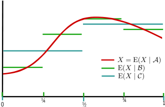
The σ-algebra ${\mathcal {H}}$ controls the "granularity" of the conditioning. A conditional expectation $E(X\mid {\mathcal {H}})$ over a finer (larger) σ-algebra ${\mathcal {H}}$ retains information about the probabilities of a larger class of events. A conditional expectation over a coarser (smaller) σ-algebra averages over more events.

Conditioning as factorization

In the definition of conditional expectation that we provided above, the fact that $Y$ is a real random element is irrelevant. Let $(U,\Sigma )$ be a measurable space, where $\Sigma$ is a σ-algebra on $U$ . A $U$ -valued random element is a measurable function $Y\colon \Omega \to U$ , i.e. $Y^{-1}(B)\in {\mathcal {F}}$ for all $B\in \Sigma$ . The distribution of $Y$ is the probability measure $P_{Y}:\Sigma \to \mathbb {R}$ defined as the pushforward measure $Y_{*}P$ , that is, such that $P_{Y}(B)=P(Y^{-1}(B))$ .

Theorem. If $X:\Omega \to \mathbb {R}$ is an integrable random variable, then there exists a unique integrable random element $\operatorname {E}(X\mid Y):U\to {\mathbb {R}}$ , defined $P_{Y}$ almost surely, such that

\int _{Y^{-1}(B)}X\,\mathrm {d} P=\int _{B}\operatorname {E} (X\mid Y)\,\mathrm {d} P_{Y},

for all $B\in \Sigma$ .

Proof sketch. Let $\mu :\Sigma \to {\mathbb {R}}$ be such that ${\textstyle \mu (B)=\int _{Y^{-1}(B)}X\,\mathrm {d} P}$ . Then $\mu$ is a signed measure which is absolutely continuous with respect to $P_{Y}$ . Indeed $P_{Y}(B)=0$ means exactly that $P(Y^{-1}(B))=0$ , and since the integral of an integrable function on a set of probability 0 is 0, this proves absolute continuity. The Radon–Nikodym theorem then proves the existence of a density of $\mu$ with respect to $P_{Y}$ . This density is $\operatorname {E}(X\mid Y)$ . $\square$

Comparing with conditional expectation with respect to sub-σ-algebras, it holds that

\operatorname{E}(X \mid Y) \circ Y= \operatorname{E}\left(X \mid Y^{-1} \left(\Sigma\right)\right).

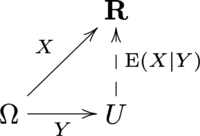
We can further interpret this equality by considering the abstract change of variables formula to transport the integral on the right hand side to an integral over Ω:

\int _{Y^{-1}(B)}X\,\mathrm {d} P=\int _{Y^{-1}(B)}(\operatorname {E} (X\mid Y)\circ Y)\,\mathrm {d} P.

The equation means that the integrals of $X$ and the composition $\operatorname {E}(X\mid Y)\circ Y$ over sets of the form $Y^{{-1}}(B)$ , for $B\in \Sigma$ , are identical.

This equation can be interpreted to say that the following diagram is commutative on average.

Computation

When X and Y are both discrete random variables, then the conditional expectation of X given the event Y = y can be considered as function of y for y in the range of Y:

\operatorname {E} (X\mid Y=y)=\sum _{x\in {\mathcal {X}}}x\,P(X=x\mid Y=y)=\sum _{x\in {\mathcal {X}}}x\,{\frac {P(X=x,Y=y)}{P(Y=y)}},

where ${\mathcal {X}}$ is the range of X.

If X is a continuous random variable, while Y remains a discrete variable, the conditional expectation is

\operatorname {E} (X\mid Y=y)=\int _{\mathcal {X}}xf_{X}(x\mid Y=y)\,\mathrm {d} x,

with $f_{X}(x\mid Y=y)={\frac {f_{X,Y}(x,y)}{P(Y=y)}}$ (where f_X,Y(x, y) gives the joint density of X and Y) being the conditional density of X given Y = y.

If both X and Y are continuous random variables, then the conditional expectation is

\operatorname {E} (X\mid Y=y)=\int _{\mathcal {X}}xf_{X\mid Y}(x\mid y)\,\mathrm {d} x,

where $f_{X\mid Y}(x\mid y)={\frac {f_{X,Y}(x,y)}{f_{Y}(y)}}$ (where f_Y(y) gives the density of Y).

Basic properties

All the following formulas are to be understood in an almost sure sense. The σ-algebra ${\mathcal {H}}$ could be replaced by a random variable $Z$ .

Pulling out independent factors:
- If $X$ is independent of ${\mathcal {H}}$ , then $E(X\mid {\mathcal {H}})=E(X)$ .

Proof

Let $B\in {\mathcal {H}}$ . Then $X$ is independent of $1_{B}$ , so we get that

\int _{B}X\,dP=E(X1_{B})=E(X)E(1_{B})=E(X)P(B)=\int _{B}E(X)\,dP.

Thus the definition of conditional expectation is satisfied by the constant random variable $E(X)$ , as desired.

- If $X$ is independent of $\sigma (Y,{\mathcal {H}})$ , then $E(XY\mid {\mathcal {H}})=E(X)\,E(Y\mid {\mathcal {H}})$ . Note that this is not necessarily the case if $X$ is only independent of ${\mathcal {H}}$ and of $Y$ .
- If $X,Y$ are independent, ${\mathcal {G}},{\mathcal {H}}$ are independent, $X$ is independent of ${\mathcal {H}}$ and $Y$ is independent of ${\mathcal {G}}$ , then $E(E(XY\mid {\mathcal {G}})\mid {\mathcal {H}})=E(X)E(Y)=E(E(XY\mid {\mathcal {H}})\mid {\mathcal {G}})$ .
Stability:
- If $X$ is ${\mathcal {H}}$ -measurable, then $E(X\mid {\mathcal {H}})=X$ .
- If Z is a random variable, then $\operatorname {E}(f(Z)\mid Z)=f(Z)$ . In its simplest form, this says $\operatorname {E}(Z\mid Z)=Z$ .
Pulling out known factors:
- If $X$ is ${\mathcal {H}}$ -measurable, then $E(XY\mid {\mathcal {H}})=X\,E(Y\mid {\mathcal {H}})$ .
- If Z is a random variable, then $\operatorname {E}(f(Z)Y\mid Z)=f(Z)\operatorname {E}(Y\mid Z)$ .
Law of total expectation: $E(E(X\mid {\mathcal {H}}))=E(X)$ .
Tower property:
- For sub-σ-algebras ${\mathcal {H}}_{1}\subset {\mathcal {H}}_{2}\subset {\mathcal {F}}$ we have $E(E(X\mid {\mathcal {H}}_{2})\mid {\mathcal {H}}_{1})=E(X\mid {\mathcal {H}}_{1})$ .
  - A special case is when Z is a ${\mathcal {H}}$ -measurable random variable. Then $\sigma (Z)\subset {\mathcal {H}}$ and thus $E(E(X\mid {\mathcal {H}})\mid Z)=E(X\mid Z)$ .
  - Doob martingale property: the above with $Z=E(X\mid {\mathcal {H}})$ (which is ${\mathcal {H}}$ -measurable), and using also $\operatorname {E}(Z\mid Z)=Z$ , gives $E(X\mid E(X\mid {\mathcal {H}}))=E(X\mid {\mathcal {H}})$ .
- For random variables $X,Y$ we have $E(E(X\mid Y)\mid f(Y))=E(X\mid f(Y))$ .
- For random variables $X,Y,Z$ we have $E(E(X\mid Y,Z)\mid Y)=E(X\mid Y)$ .
Linearity: we have $E(X_{1}+X_{2}\mid {\mathcal {H}})=E(X_{1}\mid {\mathcal {H}})+E(X_{2}\mid {\mathcal {H}})$ and $E(aX\mid {\mathcal {H}})=a\,E(X\mid {\mathcal {H}})$ for $a\in \mathbb{R}$ .
Positivity: If $X\geq 0$ then $E(X\mid {\mathcal {H}})\geq 0$ .
Monotonicity: If $X_{1}\leq X_{2}$ then $E(X_{1}\mid {\mathcal {H}})\leq E(X_{2}\mid {\mathcal {H}})$ .
Monotone convergence: If $0\leq X_{n}\uparrow X$ then $E(X_{n}\mid {\mathcal {H}})\uparrow E(X\mid {\mathcal {H}})$ .
Dominated convergence: If $X_{n}\to X$ and $|X_{n}|\leq Y$ with $Y\in L^{1}$ , then $E(X_{n}\mid {\mathcal {H}})\to E(X\mid {\mathcal {H}})$ .
Fatou's lemma: If $\textstyle E(\inf _{n}X_{n}\mid {\mathcal {H}})>-\infty$ then $\textstyle E(\liminf _{n\to \infty }X_{n}\mid {\mathcal {H}})\leq \liminf _{n\to \infty }E(X_{n}\mid {\mathcal {H}})$ .
Jensen's inequality: If $f\colon \mathbb {R} \rightarrow \mathbb {R}$ is a convex function, then $f(E(X\mid {\mathcal {H}}))\leq E(f(X)\mid {\mathcal {H}})$ .
Conditional variance: Using the conditional expectation we can define, by analogy with the definition of the variance as the mean square deviation from the average, the conditional variance
- Definition: $\operatorname {Var}(X\mid {\mathcal {H}})=\operatorname {E}{\bigl (}(X-\operatorname {E}(X\mid {\mathcal {H}}))^{2}\mid {\mathcal {H}}{\bigr )}$
- Algebraic formula for the variance: $\operatorname {Var}(X\mid {\mathcal {H}})=\operatorname {E}(X^{2}\mid {\mathcal {H}})-{\bigl (}\operatorname {E}(X\mid {\mathcal {H}}){\bigr )}^{2}$
- Law of total variance: $\operatorname {Var}(X)=\operatorname {E}(\operatorname {Var}(X\mid {\mathcal {H}}))+\operatorname {Var}(\operatorname {E}(X\mid {\mathcal {H}}))$ .
Martingale convergence: For a random variable $X$ , that has finite expectation, we have $E(X\mid {\mathcal {H}}_{n})\to E(X\mid {\mathcal {H}})$ , if either ${\mathcal {H}}_{1}\subset {\mathcal {H}}_{2}\subset \dotsb$ is an increasing series of sub-σ-algebras and $\textstyle {\mathcal {H}}=\sigma (\bigcup _{n=1}^{\infty }{\mathcal {H}}_{n})$ or if ${\mathcal {H}}_{1}\supset {\mathcal {H}}_{2}\supset \dotsb$ is a decreasing series of sub-σ-algebras and $\textstyle {\mathcal {H}}=\bigcap _{n=1}^{\infty }{\mathcal {H}}_{n}$ .
Conditional expectation as $L^{2}$ -projection: If $X,Y$ are in the Hilbert space of square-integrable real random variables (real random variables with finite second moment) then
- for ${\mathcal {H}}$ -measurable $Y$ , we have $E(Y(X-E(X\mid {\mathcal {H}})))=0$ , i.e. the conditional expectation $E(X\mid {\mathcal {H}})$ is in the sense of the L²(P) scalar product the orthogonal projection from $X$ to the linear subspace of ${\mathcal {H}}$ -measurable functions. (This allows to define and prove the existence of the conditional expectation based on the Hilbert projection theorem.)
- the mapping $X\mapsto \operatorname {E}(X\mid {\mathcal {H}})$ is self-adjoint: $\operatorname E(X\operatorname E(Y\mid {\mathcal {H}}))=\operatorname E\left(\operatorname E(X\mid {\mathcal {H}})\operatorname E(Y\mid {\mathcal {H}})\right)=\operatorname E(\operatorname E(X\mid {\mathcal {H}})Y)$
Conditioning is a contractive projection of L^p spaces $L^{p}(\Omega ,{\mathcal {F}},P)\rightarrow L^{p}(\Omega ,{\mathcal {H}},P)$ . I.e., $\operatorname {E} {\big (}|\operatorname {E} (X\mid {\mathcal {H}})|^{p}{\big )}\leq \operatorname {E} {\big (}|X|^{p}{\big )}$ for any p ≥ 1.
Doob's conditional independence property:^[6] If $X,Y$ are conditionally independent given $Z$ , then $P(X\in B\mid Y,Z)=P(X\in B\mid Z)$ (equivalently, $E(1_{\{X\in B\}}\mid Y,Z)=E(1_{\{X\in B\}}\mid Z)$ ).

Notes

↑
Kolmogorov, Andrey (1933). Grundbegriffe der Wahrscheinlichkeitsrechnung (in German). Berlin: Julius Springer. p. 46.
- Translation: Kolmogorov, Andrey (1956). Foundations of the Theory of Probability (2nd ed.). New York: Chelsea. ISBN 0-8284-0023-7.
↑ Oxtoby, J. C. (1953). "Review: Measure theory, by P. R. Halmos" (PDF). Bull. Amer. Math. Soc. 59 (1): 89–91. doi:10.1090/s0002-9904-1953-09662-8.
↑ J. L. Doob (1953). Stochastic Processes. John Wiley & Sons. ISBN 0-471-52369-0.
↑ Olav Kallenberg: Foundations of Modern Probability. 2. edition. Springer, New York 2002, ISBN 0-387-95313-2, S. 573.
↑ Billingsley, Patrick (1995). "Section 34. Conditional Expectation". Probability and Measure (3rd ed.). John Wiley & Sons. p. 445. ISBN 0-471-00710-2.
↑ Kallenberg, Olav (2001). Foundations of Modern Probability (2nd ed.). York, PA, USA: Springer. p. 110. ISBN 0-387-95313-2.

References

William Feller, An Introduction to Probability Theory and its Applications, vol 1, 1950, page 223
Paul A. Meyer, Probability and Potentials, Blaisdell Publishing Co., 1966, page 28
Grimmett, Geoffrey; Stirzaker, David (2001). Probability and Random Processes (3rd ed.). Oxford University Press. ISBN 0-19-857222-0. , pages 67–69

External links

Ushakov, N.G. (2001) [1994], "Conditional mathematical expectation", in Hazewinkel, Michiel, Encyclopedia of Mathematics, Springer Science+Business Media B.V. / Kluwer Academic Publishers, ISBN 978-1-55608-010-4

This article is issued from Wikipedia. The text is licensed under Creative Commons - Attribution - Sharealike. Additional terms may apply for the media files.

[kol1933-1] Kolmogorov, Andrey (1933). Grundbegriffe der Wahrscheinlichkeitsrechnung (in German). Berlin: Julius Springer. p. 46.
Translation: Kolmogorov, Andrey (1956). Foundations of the Theory of Probability (2nd ed.). New York: Chelsea. ISBN 0-8284-0023-7.

[mwAos] Translation: Kolmogorov, Andrey (1956). Foundations of the Theory of Probability (2nd ed.). New York: Chelsea. ISBN 0-8284-0023-7.

[halmos1950-2] Oxtoby, J. C. (1953). "Review: Measure theory, by P. R. Halmos" (PDF). Bull. Amer. Math. Soc. 59 (1): 89–91. doi:10.1090/s0002-9904-1953-09662-8.

[doob1953-3] J. L. Doob (1953). Stochastic Processes. John Wiley & Sons. ISBN 0-471-52369-0.

[4] Olav Kallenberg: Foundations of Modern Probability. 2. edition. Springer, New York 2002, ISBN 0-387-95313-2, S. 573.

[billingsley1995-5] Billingsley, Patrick (1995). "Section 34. Conditional Expectation". Probability and Measure (3rd ed.). John Wiley & Sons. p. 445. ISBN 0-471-00710-2.

[6] Kallenberg, Olav (2001). Foundations of Modern Probability (2nd ed.). York, PA, USA: Springer. p. 110. ISBN 0-387-95313-2.

Conditional expectation

Examples

History

Classical definition

Conditional expectation with respect to an event

Conditional expectation with respect to a random variable

Formal definition

Conditional expectation with respect to a sub-σ-algebra

Conditional expectation with respect to a random variable

Discussion

Conditioning as factorization

Computation

Basic properties

See also

Notes

References

External links