''q''-exponential distribution

q-exponential distribution
	Probability density function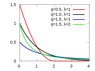
Parameters	shape (real) ; rate (real)
Support	;
PDF
CDF
Mean	; Otherwise undefined
Median
Mode	0
Variance
Skewness
Ex. kurtosis

The q-exponential distribution is a probability distribution arising from the maximization of the Tsallis entropy under appropriate constraints, including constraining the domain to be positive. It is one example of a Tsallis distribution. The q-exponential is a generalization of the exponential distribution in the same way that Tsallis entropy is a generalization of standard Boltzmann–Gibbs entropy or Shannon entropy.^[1] The exponential distribution is recovered as $q\rightarrow 1.$

Originally proposed by the statisticians George Box and David Cox in 1964,^[2] and known as the reverse Box–Cox transformation for $q=1-\lambda ,$ a particular case of power transform in statistics.

Characterization

Probability density function

The q-exponential distribution has the probability density function

(2-q)\lambda e_{q}(-\lambda x)

where

e_{q}(x)=[1+(1-q)x]^{1/(1-q)}

is the q-exponential if q ≠ 1. When q = 1, e_q(x) is just exp(x).

Derivation

In a similar procedure to how the exponential distribution can be derived using the standard Boltzmann–Gibbs entropy or Shannon entropy and constraining the domain of the variable to be positive, the q-exponential distribution can be derived from a maximization of the Tsallis Entropy subject to the appropriate constraints.

Relationship to other distributions

The q-exponential is a special case of the generalized Pareto distribution where

\mu =0,\quad \xi ={\frac {q-1}{2-q}},\quad \sigma ={\frac {1}{\lambda (2-q)}}.

The q-exponential is the generalization of the Lomax distribution (Pareto Type II), as it extends this distribution to the cases of finite support. The Lomax parameters are:

\alpha ={\frac {2-q}{q-1}},\quad \lambda _{\mathrm {Lomax} }={\frac {1}{\lambda (q-1)}}.

As the Lomax distribution is a shifted version of the Pareto distribution, the q-exponential is a shifted reparameterized generalization of the Pareto. When q > 1, the q-exponential is equivalent to the Pareto shifted to have support starting at zero. Specifically, if

X\sim \operatorname {{\mathit {q}}-Exp} (q,\lambda ){\text{ and }}Y\sim \left[\operatorname {Pareto} \left(x_{m}={\frac {1}{\lambda (q-1)}},\alpha ={\frac {2-q}{q-1}}\right)-x_{m}\right],

then $X\sim Y.$

Generating random deviates

Random deviates can be drawn using inverse transform sampling. Given a variable U that is uniformly distributed on the interval (0,1), then

X={\frac {-q'\ln _{q'}(U)}{\lambda }}\sim \operatorname {{\mathit {q}}-Exp} (q,\lambda )

where $\ln _{q'}$ is the q-logarithm and $q'={\frac {1}{2-q}}.$

Applications

Being a power transform, it is a usual technique in statistics for stabilizing the variance, making the data more normal distribution-like and improving the validity of measures of association such as the Pearson correlation between variables. It is also found in atomic physics and quantum optics, for example processes of molecular condensate creation via transition through the Feshbach resonance.^[3]

Notes

↑ Tsallis, C. Nonadditive entropy and nonextensive statistical mechanics-an overview after 20 years. Braz. J. Phys. 2009, 39, 337–356
↑ Box, George E. P.; Cox, D. R. (1964). "An analysis of transformations". Journal of the Royal Statistical Society, Series B. 26 (2): 211–252. JSTOR 2984418. MR 0192611.
↑ C. Sun; N. A. Sinitsyn (2016). "Landau-Zener extension of the Tavis-Cummings model: Structure of the solution". Phys. Rev. A. 94 (3): 033808. arXiv:1606.08430. Bibcode:2016PhRvA..94c3808S. doi:10.1103/PhysRevA.94.033808.

External links

Tsallis Statistics, Statistical Mechanics for Non-extensive Systems and Long-Range Interactions

This article is issued from Wikipedia. The text is licensed under Creative Commons - Attribution - Sharealike. Additional terms may apply for the media files.

[1] Tsallis, C. Nonadditive entropy and nonextensive statistical mechanics-an overview after 20 years. Braz. J. Phys. 2009, 39, 337–356

[boxcox-2] Box, George E. P.; Cox, D. R. (1964). "An analysis of transformations". Journal of the Royal Statistical Society, Series B. 26 (2): 211–252. JSTOR 2984418. MR 0192611.

[sun-16pra2-3] C. Sun; N. A. Sinitsyn (2016). "Landau-Zener extension of the Tavis-Cummings model: Structure of the solution". Phys. Rev. A. 94 (3): 033808. arXiv:1606.08430. Bibcode:2016PhRvA..94c3808S. doi:10.1103/PhysRevA.94.033808.

Probability distributions
List
Discrete univariate with finite support	Benford Bernoulli beta-binomial binomial categorical hypergeometric Poisson binomial Rademacher discrete uniform Zipf Zipf–Mandelbrot
Discrete univariate with infinite support	beta negative binomial Borel Conway–Maxwell–Poisson discrete phase-type Delaporte extended negative binomial Gauss–Kuzmin geometric logarithmic negative binomial parabolic fractal Poisson Skellam Yule–Simon zeta
Continuous univariate supported on a bounded interval	arcsine ARGUS Balding–Nichols Bates beta beta rectangular Irwin–Hall Kumaraswamy logit-normal noncentral beta raised cosine reciprocal triangular U-quadratic uniform Wigner semicircle
Continuous univariate supported on a semi-infinite interval	Benini Benktander 1st kind Benktander 2nd kind beta prime Burr chi-squared chi Dagum Davis exponential-logarithmic Erlang exponential F folded normal Flory–Schulz Fréchet gamma gamma/Gompertz generalized inverse Gaussian Gompertz half-logistic half-normal Hotelling's T-squared hyper-Erlang hyperexponential hypoexponential inverse chi-squared scaled inverse chi-squared inverse Gaussian inverse gamma Kolmogorov Lévy log-Cauchy log-Laplace log-logistic log-normal Lomax matrix-exponential Maxwell–Boltzmann Maxwell–Jüttner Mittag-Leffler Nakagami noncentral chi-squared Pareto phase-type poly-Weibull Rayleigh relativistic Breit–Wigner Rice shifted Gompertz truncated normal type-2 Gumbel Weibull Discrete Weibull Wilks's lambda
Continuous univariate supported on the whole real line	Cauchy exponential power Fisher's z Gaussian q generalized normal generalized hyperbolic geometric stable Gumbel Holtsmark hyperbolic secant Johnson's S_U Landau Laplace asymmetric Laplace logistic noncentral t normal (Gaussian) normal-inverse Gaussian skew normal slash stable Student's t type-1 Gumbel Tracy–Widom variance-gamma Voigt
Continuous univariate with support whose type varies	generalized extreme value generalized Pareto Marchenko–Pastur q-exponential q-Gaussian q-Weibull shifted log-logistic Tukey lambda
Mixed continuous-discrete univariate	rectified Gaussian
Multivariate (joint)	Discrete Ewens multinomial Dirichlet-multinomial negative multinomial Continuous Dirichlet generalized Dirichlet multivariate Laplace multivariate normal multivariate stable multivariate t normal-inverse-gamma normal-gamma Matrix-valued inverse matrix gamma inverse-Wishart matrix normal matrix t matrix gamma normal-inverse-Wishart normal-Wishart Wishart
Directional	Univariate (circular) directional Circular uniform univariate von Mises wrapped normal wrapped Cauchy wrapped exponential wrapped asymmetric Laplace wrapped Lévy Bivariate (spherical) Kent Bivariate (toroidal) bivariate von Mises Multivariate von Mises–Fisher Bingham
Degenerate and singular	Degenerate Dirac delta function Singular Cantor
Families	Circular compound Poisson elliptical exponential natural exponential location–scale maximum entropy mixture Pearson Tweedie wrapped