Probability mass function

The graph of a probability mass function. All the values of this function must be non-negative and sum up to 1.

In probability and statistics, a probability mass function (pmf) is a function that gives the probability that a discrete random variable is exactly equal to some value.^[1] The probability mass function is often the primary means of defining a discrete probability distribution, and such functions exist for either scalar or multivariate random variables whose domain is discrete.

A probability mass function differs from a probability density function (pdf) in that the latter is associated with continuous rather than discrete random variables; the values of the probability density function are not probabilities as such: a pdf must be integrated over an interval to yield a probability.^[2]

The value of the random variable having the largest probability mass is called the mode.

Formal definition

Suppose that X: S → A (A $\subseteq$ R) is a discrete random variable defined on a sample space S. Then the probability mass function f_X: A → [0, 1] for X is defined as^[3]^[4]

f_{X}(x)=\Pr(X=x)=P(\{s\in S:X(s)=x\}).

Thinking of probability as mass helps to avoid mistakes since the physical mass is conserved as is the total probability for all hypothetical outcomes x:

\sum _{x\in A}f_{X}(x)=1

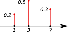
When there is a natural order among the potential outcomes x, it may be convenient to assign numerical values to them (or n-tuples in case of a discrete multivariate random variable) and to consider also values not in the image of X. That is, f_X may be defined for all real numbers and f_X(x) = 0 for all x $\notin$ X(S) as shown in the figure.

Since the image of X is countable, the probability mass function f_X(x) is zero for all but a countable number of values of x. The discontinuity of probability mass functions is related to the fact that the cumulative distribution function of a discrete random variable, when it is meaningful because there is a natural ordering, is also discontinuous. Where it is differentiable, the derivative is zero, just as the probability mass function is zero at all such points.

Measure theoretic formulation

A probability mass function of a discrete random variable X can be seen as a special case of two more general measure theoretic constructions: the distribution of X and the probability density function of X with respect to the counting measure. We make this more precise below.

Suppose that $(A,{\mathcal {A}},P)$ is a probability space and that $(B,{\mathcal {B}})$ is a measurable space whose underlying σ-algebra is discrete, so in particular contains singleton sets of B. In this setting, a random variable $X\colon A\to B$ is discrete provided its image is countable. The pushforward measure $X_{*}(P)$ —called a distribution of X in this context—is a probability measure on B whose restriction to singleton sets induces a probability mass function $f_{X}\colon B\to \mathbb {R}$ since $f_{X}(b)=P(X^{-1}(b))=[X_{*}(P)](\{b\})$ for each b in B.

Now suppose that $(B,{\mathcal {B}},\mu )$ is a measure space equipped with the counting measure μ. The probability density function f of X with respect to the counting measure, if it exists, is the Radon–Nikodym derivative of the pushforward measure of X (with respect to the counting measure), so $f=dX_{*}P/d\mu$ and f is a function from B to the non-negative reals. As a consequence, for any b in B we have

P(X=b)=P(X^{-1}(\{b\})):=\int _{X^{-1}(\{b\})}dP=

\int _{\{b\}}fd\mu =f(b),

demonstrating that f is in fact a probability mass function.

Examples

Finite

The probability mass function of a fair die. All the numbers on the die have an equal chance of appearing on top when the die stops rolling.

If the discrete distribution has two or more categories one of which may occur, whether or not these categories have a natural ordering, when there is only a single trial (draw) this is a categorical distribution.

Suppose that S is the sample space of all outcomes of a single toss of a fair coin, and X is the random variable defined on S assigning 0 to the category "tails" and 1 to the category "heads". Since the coin is fair, the probability mass function is

f_{X}(x)={\begin{cases}{\frac {1}{2}},&x\in \{0,1\},\\0,&x\notin \{0,1\}.\end{cases}}

This is a special case of the binomial distribution, the Bernoulli distribution.

An example of a multivariate discrete distribution, and of its probability mass function, is provided by the multinomial distribution. Here the multiple random variables are the numbers of successes in each of the categories after a given number of trials, and each non-zero probability mass gives the probability of a certain combination of numbers of successes in the various categories.

Countably infinite

The following exponentially declining distribution is an example of a distribution with an infinite number of possible outcomes—all the positive integers:

{\text{Pr}}(X=i)={\frac {1}{2^{i}}}\quad {\text{for}}\quad i=1,2,3,\dots .

Despite the infinite number of possible outcomes, the total probability mass is 1/2 + 1/4 + 1/8 + ... = 1, satisfying the unit total probability requirement for a probability distribution.

Multivariate case

Two or more discrete random variables have a joint probability mass function, which gives the probability of each possible combination of realizations for the random variables.

References

↑ Stewart, William J. (2011). Probability, Markov Chains, Queues, and Simulation: The Mathematical Basis of Performance Modeling. Princeton University Press. p. 105. ISBN 978-1-4008-3281-1.
↑ Probability Function at Mathworld
↑ Kumar, Dinesh (2006). Reliability & Six Sigma. Birkhäuser. p. 22. ISBN 978-0-387-30255-3.
↑ Rao, S.S. (1996). Engineering optimization: theory and practice. John Wiley & Sons. p. 717. ISBN 978-0-471-55034-1.

Theory of probability distributions
probability mass function (pmf) probability density function (pdf) cumulative distribution function (cdf) quantile function
raw moment central moment mean variance standard deviation skewness kurtosis L-moment
moment-generating function (mgf) characteristic function probability-generating function (pgf) cumulant combinant