Generalized extreme value distribution

Notation
Parameters	μ ∈ R — location,; σ > 0 — scale,; ξ ∈ R — shape.
Support	x ∈ [ μ − σ / ξ, +∞) when ξ > 0,; x ∈ (−∞, +∞) when ξ = 0,; x ∈ (−∞, μ − σ / ξ ] when ξ < 0.
PDF	where
CDF	for x ∈ support
Mean	where gk = Γ(1 − kξ), ; and is Euler’s constant.
Median
Mode
Variance	.
Skewness	; where is the sign function ; and is the Riemann zeta function
Ex. kurtosis
Entropy
MGF	[1]
CF	[1]

In probability theory and statistics, the generalized extreme value (GEV) distribution is a family of continuous probability distributions developed within extreme value theory to combine the Gumbel, Fréchet and Weibull families also known as type I, II and III extreme value distributions. By the extreme value theorem the GEV distribution is the only possible limit distribution of properly normalized maxima of a sequence of independent and identically distributed random variables. Note that a limit distribution need not exist: this requires regularity conditions on the tail of the distribution. Despite this, the GEV distribution is often used as an approximation to model the maxima of long (finite) sequences of random variables.

In some fields of application the generalized extreme value distribution is known as the Fisher–Tippett distribution, named after Ronald Fisher and L. H. C. Tippett who recognised three different forms outlined below. However usage of this name is sometimes restricted to mean the special case of the Gumbel distribution. The common functional form for all 3 distributions was discovered by McFadden in 1978.^[2]

Specification

Using the standardized variable $s=(x-\mu )/\sigma$ , where $\mu\in\mathbb R$ is the location parameter and $\sigma >0$ is the scale parameter, the cumulative distribution function of the GEV distribution is

F(s;\xi )={\begin{cases}\exp(-(1+\xi s)^{-1/\xi })&\xi \neq 0\\\exp(-\exp(-s))&\xi =0\end{cases}}

where $\xi\in\mathbb R$ is the shape parameter. Thus for $\xi>0$ , the expression is valid for $s>-1/\xi$ , while for $\xi<0$ it is valid for $s<-1/\xi$ . In the first case, at the lower end-point, it equals 0; in the second case, at the upper end-point, it equals 1. For $\xi = 0$ the first expression is formally undefined and is replaced with the result obtained by taking the limit as $\xi\to 0$ in which case $s\in \mathbb {R}$ .

If $x=\mu$ then $s=0$ and $F(s;\xi )=exp(-1)$ ≈ $0.37$ whatever the values of $\xi$ and $\sigma .$

The probability density function of the standardized distribution is

f(s;\xi )={\begin{cases}(1+\xi s)^{(-1/\xi )-1}\exp(-(1+\xi s)^{-1/\xi })&\xi \neq 0\\\exp(-s)\exp(-\exp(-s))&\xi =0\end{cases}}

again valid for $s>-1/\xi$ in the case $\xi>0$ , and for $s<-1/\xi$ in the case $\xi<0$ . The density is zero outside of the relevant range. In the case $\xi =0$ the density is positive on the whole real line.

Since the cumulative distribution function is invertible, the quantile function for the GEV distribution has an explicit expression, namely

Q(p;\mu ,\sigma ,\xi )={\begin{cases}\mu +\sigma ((-\log(p))^{-\xi }-1)/\xi &\xi >0\,\,{\textrm {and}}\,\,p\in [0,1);\,\xi <0\,\,{\textrm {and}}\,\,p\in (0,1]\\\mu -\sigma \log(-\log(p))&\xi =0,\,p\in (0,1),\end{cases}}

and therefore the quantile density function $(q=dQ/dp)$ is

q(p;\sigma ,\xi )={\frac {\sigma }{p(-\log(p))^{\xi +1}}}.

Summary statistics

Some simple statistics of the distribution are:

\operatorname {E} (X)=\mu -{\frac {\sigma }{\xi }}+{\frac {\sigma }{\xi }}g_{1}

for

\xi <1

\operatorname{Var}(X) = \frac{\sigma^2}{\xi^2}(g_2-g_1^2) ,

\operatorname{Mode}(X) = \mu+\frac{\sigma}{\xi}[(1+\xi)^{-\xi}-1] .

The skewness is for ξ>0

\operatorname {skewness} (X)={\frac {g_{3}-3g_{2}g_{1}+2g_{1}^{3}}{(g_{2}-g_{1}^{2})^{3/2}}}

For ξ<0, the sign of the numerator is reversed.

The excess kurtosis is:

\operatorname {kurtosis\ excess} (X)={\frac {g_{4}-4g_{3}g_{1}+6g_{2}g_{1}^{2}-3g_{1}^{4}}{(g_{2}-g_{1}^{2})^{2}}}-3.

where $g_k=\Gamma(1-k\xi)$ , k=1,2,3,4, and $\Gamma(t)$ is the gamma function.

Link to Fréchet, Weibull and Gumbel families

The shape parameter $\xi$ governs the tail behavior of the distribution. The sub-families defined by $\xi= 0$ , $\xi>0$ and $\xi<0$ correspond, respectively, to the Gumbel, Fréchet and Weibull families, whose cumulative distribution functions are displayed below.

Gumbel or type I extreme value distribution ( $\xi =0$ )

F(x;\mu,\sigma,0)=e^{-e^{-(x-\mu)/\sigma}}\;\;\; \text{for} \;\; x\in\mathbb R.

Fréchet or type II extreme value distribution, if $\xi=\alpha^{-1}>0$ and $y = 1 + \xi (x-\mu)/\sigma$

F(x;\mu,\sigma,\xi)=\begin{cases} e^{-y^{-\alpha}} & y > 0 \\ 0 & y \leq 0. \end{cases}

Reversed Weibull or type III extreme value distribution, if $\xi=-\alpha^{-1}<0$ and $y=-\left(1+\xi (x-\mu )/\sigma \right)$

F(x;\mu,\sigma,\xi)=\begin{cases} e^{-(-y)^{\alpha}} & y<0 \\ 1 & y\geq 0 \end{cases}

Remark I: The theory here relates to maxima and the distribution being discussed is an extreme value distribution for maxima. A generalised extreme value distribution for minima can be obtained, for example by substituting (−x) for x in the distribution function, and subtracting from one: this yields a separate family of distributions.

Remark II: The ordinary Weibull distribution arises in reliability applications and is obtained from the distribution here by using the variable $t = \mu - x$ , which gives a strictly positive support - in contrast to the use in the extreme value theory here. This arises because the Weibull distribution is used in cases that deal with the minimum rather than the maximum. The distribution here has an addition parameter compared to the usual form of the Weibull distribution and, in addition, is reversed so that the distribution has an upper bound rather than a lower bound. Importantly, in applications of the GEV, the upper bound is unknown and so must be estimated, while when applying the Weibull distribution the lower bound is known to be zero.

Remark III: Note the differences in the ranges of interest for the three extreme value distributions: Gumbel is unlimited, Fréchet has a lower limit, while the reversed Weibull has an upper limit. More precisely, Extreme Value Theory (Univariate Theory) describes which of the three is the limiting law according to the initial law X and in particular depending on its tail (e.g. maximum distribution of a heavy tailed law converges to Fréchet).

One can link the type I to types II and III the following way: if the cumulative distribution function of some random variable $X$ is of type II, and with the positive numbers as support, i.e. $F(x; 0, \sigma, \alpha)$ , then the cumulative distribution function of $\ln X$ is of type I, namely $F(x; \ln \sigma, 1/\alpha, 0)$ . Similarly, if the cumulative distribution function of $X$ is of type III, and with the negative numbers as support, i.e. $F(x; 0, \sigma, -\alpha)$ , then the cumulative distribution function of $\ln (-X)$ is of type I, namely $F(x; -\ln \sigma, 1/\alpha, 0)$ .

Link to logit models (logistic regression)

Multinomial logit models, and certain other types of logistic regression, can be phrased as latent variable models with error variables distributed as Gumbel distributions (type I generalized extreme value distributions). This phrasing is common in the theory of discrete choice models, which include logit models, probit models, and various extensions of them, and derives from the fact that the difference of two type-I GEV-distributed variables follows a logistic distribution, of which the logit function is the quantile function. The type-I GEV distribution thus plays the same role in these logit models as the normal distribution does in the corresponding probit models.

Properties

The cumulative distribution function of the generalized extreme value distribution solves the stability postulate equation. The generalized extreme value distribution is a special case of a max-stable distribution, and is a transformation of a min-stable distribution.

Applications

The GEV distribution is widely used in the treatment of "tail risks" in fields ranging from insurance to finance. In the latter case, it has been considered as a means of assessing various financial risks via metrics such as Value at Risk.^[3]^[4]

Fitted GEV probability distribution to monthly maximum one-day rainfalls in October, Surinam^[5]

However, the resulting shape parameters have been found to lie in the range leading to undefined means and variances, which underlines the fact that reliable data analysis is often impossible.^[6]

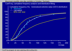
In hydrology the GEV distribution is applied to extreme events such as annual maximum one-day rainfalls and river discharges. The blue picture, made with CumFreq, illustrates an example of fitting the GEV distribution to ranked annually maximum one-day rainfalls showing also the 90% confidence belt based on the binomial distribution. The rainfall data are represented by plotting positions as part of the cumulative frequency analysis.

Related distributions

If $X \sim \textrm{GEV}(\mu,\,\sigma,\,0)$ then $mX+b \sim \textrm{GEV}(m\mu+b,\,m\sigma,\,0)$
If $X \sim \textrm{Gumbel}(\mu,\,\sigma)$ (Gumbel distribution) then $X \sim \textrm{GEV}(\mu,\,\sigma,\,0)$
If $X \sim \textrm{Weibull}(\sigma,\,\mu)$ (Weibull distribution) then $\mu\left(1-\sigma\mathrm{log}{\tfrac{X}{\sigma}}\right) \sim \textrm{GEV}(\mu,\,\sigma,\,0)$
If $X \sim \textrm{GEV}(\mu,\,\sigma,\,0)$ then $\sigma \exp (-\tfrac{X-\mu}{\mu \sigma} ) \sim \textrm{Weibull}(\sigma,\,\mu)$ (Weibull distribution)
If $X \sim \textrm{Exponential}(1)\,$ (Exponential distribution) then $\mu - \sigma \log{X} \sim \textrm{GEV}(\mu,\,\sigma,\,0)$
If $X \sim \mathrm{GEV}(\alpha,\beta,0)\,$ and $Y \sim \mathrm{GEV}(\alpha,\beta,0)\,$ then $X-Y \sim \mathrm{Logistic}(0,\beta) \,$ (Logistic distribution)
If $X \sim \mathrm{GEV}(\alpha,\beta,0)\,$ and $Y \sim \mathrm{GEV}(\alpha,\beta,0)\,$ then $X+Y \sim \mathrm{Logistic}(2 \alpha,\beta) \,$

Notes

1 2 Muraleedharan. G, C. Guedes Soares and Cláudia Lucas (2011). "Characteristic and Moment Generating Functions of Generalised Extreme Value Distribution (GEV)". In Linda. L. Wright (Ed.), Sea Level Rise, Coastal Engineering, Shorelines and Tides, Chapter-14, pp. 269–276. Nova Science Publishers. ISBN 978-1-61728-655-1
↑ McFadden, Daniel (1978). "Modeling the Choice of Residential Location" (PDF). Transportation Research Record (673): 72–77.
↑ Moscadelli, Marco. "The modelling of operational risk: experience with the analysis of the data collected by the Basel Committee." Available at SSRN 557214 (2004).
↑ Guégan, D.; Hassani, B.K. (2014), "A mathematical resurgence of risk management: an extreme modeling of expert opinions", Frontiers in Finance and Economics, 11 (1): 25–45, SSRN 2558747
↑ CumFreq for probability distribution fitting
↑ Kjersti Aas, lecture, NTNU, Trondheim, 23 Jan 2008

References

Embrechts, Paul; Klüppelberg, Claudia; Mikosch, Thomas (1997). Modelling extremal events for insurance and finance. Berlin: Springer Verlag.
Leadbetter, M.R., Lindgren, G. and Rootzén, H. (1983). Extremes and related properties of random sequences and processes. Springer-Verlag. ISBN 0-387-90731-9.
Resnick, S.I. (1987). Extreme values, regular variation and point processes. Springer-Verlag. ISBN 0-387-96481-9.
Coles, Stuart (2001). An Introduction to Statistical Modeling of Extreme Values,. Springer-Verlag. ISBN 1-85233-459-2.

This article is issued from Wikipedia. The text is licensed under Creative Commons - Attribution - Sharealike. Additional terms may apply for the media files.

[R1-1] 1 2 Muraleedharan. G, C. Guedes Soares and Cláudia Lucas (2011). "Characteristic and Moment Generating Functions of Generalised Extreme Value Distribution (GEV)". In Linda. L. Wright (Ed.), Sea Level Rise, Coastal Engineering, Shorelines and Tides, Chapter-14, pp. 269–276. Nova Science Publishers. ISBN 978-1-61728-655-1

[mcfadden1978modeling-2] McFadden, Daniel (1978). "Modeling the Choice of Residential Location" (PDF). Transportation Research Record (673): 72–77.

[3] Moscadelli, Marco. "The modelling of operational risk: experience with the analysis of the data collected by the Basel Committee." Available at SSRN 557214 (2004).

[4] Guégan, D.; Hassani, B.K. (2014), "A mathematical resurgence of risk management: an extreme modeling of expert opinions", Frontiers in Finance and Economics, 11 (1): 25–45, SSRN 2558747

[5] CumFreq for probability distribution fitting

[6] Kjersti Aas, lecture, NTNU, Trondheim, 23 Jan 2008

Probability distributions
List
Discrete univariate with finite support	Benford Bernoulli beta-binomial binomial categorical hypergeometric Poisson binomial Rademacher discrete uniform Zipf Zipf–Mandelbrot
Discrete univariate with infinite support	beta negative binomial Borel Conway–Maxwell–Poisson discrete phase-type Delaporte extended negative binomial Gauss–Kuzmin geometric logarithmic negative binomial parabolic fractal Poisson Skellam Yule–Simon zeta
Continuous univariate supported on a bounded interval	arcsine ARGUS Balding–Nichols Bates beta beta rectangular Irwin–Hall Kumaraswamy logit-normal noncentral beta raised cosine reciprocal triangular U-quadratic uniform Wigner semicircle
Continuous univariate supported on a semi-infinite interval	Benini Benktander 1st kind Benktander 2nd kind beta prime Burr chi-squared chi Dagum Davis exponential-logarithmic Erlang exponential F folded normal Flory–Schulz Fréchet gamma gamma/Gompertz generalized inverse Gaussian Gompertz half-logistic half-normal Hotelling's T-squared hyper-Erlang hyperexponential hypoexponential inverse chi-squared scaled inverse chi-squared inverse Gaussian inverse gamma Kolmogorov Lévy log-Cauchy log-Laplace log-logistic log-normal Lomax matrix-exponential Maxwell–Boltzmann Maxwell–Jüttner Mittag-Leffler Nakagami noncentral chi-squared Pareto phase-type poly-Weibull Rayleigh relativistic Breit–Wigner Rice shifted Gompertz truncated normal type-2 Gumbel Weibull Discrete Weibull Wilks's lambda
Continuous univariate supported on the whole real line	Cauchy exponential power Fisher's z Gaussian q generalized normal generalized hyperbolic geometric stable Gumbel Holtsmark hyperbolic secant Johnson's S_U Landau Laplace asymmetric Laplace logistic noncentral t normal (Gaussian) normal-inverse Gaussian skew normal slash stable Student's t type-1 Gumbel Tracy–Widom variance-gamma Voigt
Continuous univariate with support whose type varies	generalized extreme value generalized Pareto Marchenko–Pastur q-exponential q-Gaussian q-Weibull shifted log-logistic Tukey lambda
Mixed continuous-discrete univariate	rectified Gaussian
Multivariate (joint)	Discrete Ewens multinomial Dirichlet-multinomial negative multinomial Continuous Dirichlet generalized Dirichlet multivariate Laplace multivariate normal multivariate stable multivariate t normal-inverse-gamma normal-gamma Matrix-valued inverse matrix gamma inverse-Wishart matrix normal matrix t matrix gamma normal-inverse-Wishart normal-Wishart Wishart
Directional	Univariate (circular) directional Circular uniform univariate von Mises wrapped normal wrapped Cauchy wrapped exponential wrapped asymmetric Laplace wrapped Lévy Bivariate (spherical) Kent Bivariate (toroidal) bivariate von Mises Multivariate von Mises–Fisher Bingham
Degenerate and singular	Degenerate Dirac delta function Singular Cantor
Families	Circular compound Poisson elliptical exponential natural exponential location–scale maximum entropy mixture Pearson Tweedie wrapped

Notation	$\textrm{GEV}(\mu,\,\sigma,\,\xi)$
Parameters	μ ∈ R — location, σ > 0 — scale, ξ ∈ R — shape.
Support	x ∈ [ μ − σ / ξ, +∞) when ξ > 0, x ∈ (−∞, +∞) when ξ = 0, x ∈ (−∞, μ − σ / ξ ] when ξ < 0.
PDF	$\frac{1}{\sigma}\,t(x)^{\xi+1}e^{-t(x)},$ where $t(x)={\begin{cases}{\big (}1+\xi ({\tfrac {x-\mu }{\sigma }}){\big )}^{-1/\xi }&{\textrm {if}}\ \xi \neq 0\\e^{-(x-\mu )/\sigma }&{\textrm {if}}\ \xi =0\end{cases}}$
CDF	$e^{-t(x)},\,$ for x ∈ support
Mean	${\begin{cases}\mu +\sigma (g_{1}-1)/\xi &{\text{if}}\ \xi \neq 0,\xi <1,\\\mu +\sigma \,\gamma &{\text{if}}\ \xi =0,\\\infty &{\text{if}}\ \xi \geq 1,\end{cases}}$ where g_k = Γ(1 − kξ), and $\gamma$ is Euler’s constant.
Median	$\begin{cases}\mu + \sigma \frac{(\ln2)^{-\xi}-1}{\xi} & \text{if}\ \xi\neq0,\\ \mu - \sigma \ln\ln2 & \text{if}\ \xi=0.\end{cases}$
Mode	$\begin{cases}\mu + \sigma \frac{(1+\xi)^{-\xi}-1}{\xi} & \text{if}\ \xi\neq0,\\ \mu & \text{if}\ \xi=0.\end{cases}$
Variance	$\begin{cases}\sigma^2\,(g_2-g_1^2)/\xi^2 & \text{if}\ \xi\neq0,\xi<\frac12,\\ \sigma^2\,\frac{\pi^2}{6} & \text{if}\ \xi=0, \\ \infty & \text{if}\ \xi\geq\frac12,\end{cases}$ .
Skewness	${\begin{cases}\operatorname {sgn}(\xi ){\frac {g_{3}-3g_{2}g_{1}+2g_{1}^{3}}{(g_{2}-g_{1}^{2})^{3/2}}}&{\text{if}}\ \xi \neq 0,\xi <{\frac {1}{3}},\\{\frac {12{\sqrt {6}}\,\zeta (3)}{\pi ^{3}}}&{\text{if}}\ \xi =0,\\\infty &{\text{if}}\ \xi \geq {\frac {1}{3}}.\end{cases}}$ where $\operatorname {sgn}(x)$ is the sign function and $\zeta (x)$ is the Riemann zeta function
Ex. kurtosis	${\begin{cases}{\frac {g_{4}-4g_{3}g_{1}-3g_{2}^{2}+12g_{2}g_{1}^{2}-6g_{1}^{4}}{(g_{2}-g_{1}^{2})^{2}}}&{\text{if}}\ \xi \neq 0,\xi <{\frac {1}{4}},\\{\frac {12}{5}}&{\text{if}}\ \xi =0,\\\infty &{\text{if}}\ \xi \geq {\frac {1}{4}}.\end{cases}}$
Entropy	$\log(\sigma )\,+\,\gamma \xi \,+\,\gamma \,+\,1$
MGF	^[1]
CF	^[1]