Kernel density estimation

Let (x₁, x₂, …, x_n) be a univariate independent and identically distributed sample drawn from some distribution with an unknown density ƒ. We are interested in estimating the shape of this function ƒ. Its kernel density estimator is

${\displaystyle {\widehat {f}}_{h}(x)={\frac {1}{n}}\sum _{i=1}^{n}K_{h}(x-x_{i})={\frac {1}{nh}}\sum _{i=1}^{n}K{\Big (}{\frac {x-x_{i}}{h}}{\Big )},}$

where K is the kernel — a non-negative function — and h > 0 is a smoothing parameter called the bandwidth. A kernel with subscript h is called the scaled kernel and defined as K_h(x) = 1/h K(x/h). Intuitively one wants to choose h as small as the data will allow; however, there is always a trade-off between the bias of the estimator and its variance. The choice of bandwidth is discussed in more detail below.

A range of kernel functions are commonly used: uniform, triangular, biweight, triweight, Epanechnikov, normal, and others. The Epanechnikov kernel is optimal in a mean square error sense,[5] though the loss of efficiency is small for the kernels listed previously.[6] Due to its convenient mathematical properties, the normal kernel is often used, which means K(x) = ϕ(x), where ϕ is the standard normal density function.

The construction of a kernel density estimate finds interpretations in fields outside of density estimation.[7] For example, in thermodynamics, this is equivalent to the amount of heat generated when heat kernels (the fundamental solution to the heat equation) are placed at each data point locations x_i. Similar methods are used to construct discrete Laplace operators on point clouds for manifold learning (e.g. diffusion map).

Kernel density estimates are closely related to histograms, but can be endowed with properties such as smoothness or continuity by using a suitable kernel. To see this, we compare the construction of histogram and kernel density estimators, using these 6 data points:

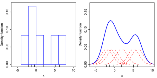
For the histogram, first the horizontal axis is divided into sub-intervals or bins which cover the range of the data. In this case, we have six bins each of width 2. Whenever a data point falls inside this interval, we place a box of height 1/12. If more than one data point falls inside the same bin, we stack the boxes on top of each other.

For the kernel density estimate, we place a normal kernel with standard deviation 2.25 (indicated by the red dashed lines) on each of the data points x_i. The kernels are summed to make the kernel density estimate (solid blue curve). The smoothness of the kernel density estimate is evident compared to the discreteness of the histogram, as kernel density estimates converge faster to the true underlying density for continuous random variables.[8]

Comparison of the histogram (left) and kernel density estimate (right) constructed using the same data. The six individual kernels are the red dashed curves, the kernel density estimate the blue curves. The data points are the rug plot on the horizontal axis.

Kernel density estimate (KDE) with different bandwidths of a random sample of 100 points from a standard normal distribution. Grey: true density (standard normal). Red: KDE with h=0.05. Black: KDE with h=0.337. Green: KDE with h=2.

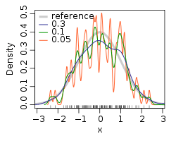
The bandwidth of the kernel is a free parameter which exhibits a strong influence on the resulting estimate. To illustrate its effect, we take a simulated random sample from the standard normal distribution (plotted at the blue spikes in the rug plot on the horizontal axis). The grey curve is the true density (a normal density with mean 0 and variance 1). In comparison, the red curve is undersmoothed since it contains too many spurious data artifacts arising from using a bandwidth h = 0.05, which is too small. The green curve is oversmoothed since using the bandwidth h = 2 obscures much of the underlying structure. The black curve with a bandwidth of h = 0.337 is considered to be optimally smoothed since its density estimate is close to the true density. An extreme situation is encountered in the limit ${\displaystyle h\to 0}$ (no smoothing), where the estimate is a sum of n delta functions centered at the coordinates of analyzed samples. In the other extreme limit ${\displaystyle h\to \infty }$ the estimate retains the shape of the used kernel, centered on the mean of the samples (completely smooth).

The most common optimality criterion used to select this parameter is the expected L₂ risk function, also termed the mean integrated squared error:

${\displaystyle \operatorname {MISE} (h)=\operatorname {E} \!\left[\,\int ({\hat {f}}_{h}(x)-f(x))^{2}\,dx\right].}$

Under weak assumptions on ƒ and K, (ƒ is the, generally unknown, real density function),[1][2] MISE (h) = AMISE(h) + o(1/(nh) + h⁴) where o is the little o notation. The AMISE is the Asymptotic MISE which consists of the two leading terms

${\displaystyle \operatorname {AMISE} (h)={\frac {R(K)}{nh}}+{\frac {1}{4}}m_{2}(K)^{2}h^{4}R(f'')}$

where ${\displaystyle R(g)=\int g(x)^{2}\,dx}$ for a function g, ${\displaystyle m_{2}(K)=\int x^{2}K(x)\,dx}$ and ƒ'' is the second derivative of ƒ. The minimum of this AMISE is the solution to this differential equation

${\displaystyle {\frac {\partial }{\partial h}}\operatorname {AMISE} (h)=-{\frac {R(K)}{nh^{2}}}+m_{2}(K)^{2}h^{3}R(f'')=0}$

or

${\displaystyle h_{\operatorname {AMISE} }={\frac {R(K)^{1/5}}{m_{2}(K)^{2/5}R(f'')^{1/5}n^{1/5}}}.}$

Neither the AMISE nor the h_AMISE formulas are able to be used directly since they involve the unknown density function ƒ or its second derivative ƒ'', so a variety of automatic, data-based methods have been developed for selecting the bandwidth. Many review studies have been carried out to compare their efficacies,[9][10][11][12][13][14][15] with the general consensus that the plug-in selectors[7] [16] and cross validation selectors[17][18][19] are the most useful over a wide range of data sets.

Substituting any bandwidth h which has the same asymptotic order n^−1/5 as h_AMISE into the AMISE gives that AMISE(h) = O(n^−4/5), where O is the big o notation. It can be shown that, under weak assumptions, there cannot exist a non-parametric estimator that converges at a faster rate than the kernel estimator.[20] Note that the n^−4/5 rate is slower than the typical n⁻¹ convergence rate of parametric methods.

If the bandwidth is not held fixed, but is varied depending upon the location of either the estimate (balloon estimator) or the samples (pointwise estimator), this produces a particularly powerful method termed adaptive or variable bandwidth kernel density estimation.

Bandwidth selection for kernel density estimation of heavy-tailed distributions is relatively difficult.[21]

A rule-of-thumb bandwidth estimator

If Gaussian basis functions are used to approximate univariate data, and the underlying density being estimated is Gaussian, the optimal choice for h (that is, the bandwidth that minimises the mean integrated squared error) is[22]:

${\displaystyle h=\left({\frac {4{\hat {\sigma }}^{5}}{3n}}\right)^{\frac {1}{5}}\approx 1.06{\hat {\sigma }}n^{-1/5},}$

In order to make the h value more robust to make the fitness well for both long-tailed and skew distribution and bimodal mixture distribution, it is better to substitute the value of ${\displaystyle {\hat {\sigma }}}$ with another parameter A, which is given by:

A=min(standard deviation, interquantile range/1.34).

Another modification that will improve the model is to reduce the factor from 1.06 to 0.9. Then the final formula would be:

${\displaystyle h=0.9*\min \left({\hat {\sigma }},{\frac {IQR}{1.34}}\right)*n^{-{\frac {1}{5}}}}$

where ${\displaystyle {\hat {\sigma }}}$ is the standard deviation of the samples, n is the sample size. IQR is the interquartile range. This approximation is termed the normal distribution approximation, Gaussian approximation, or Silverman's (1986) rule of thumb. While this rule of thumb is easy to compute, it should be used with caution as it can yield widely inaccurate estimates when the density is not close to being normal. For example, consider estimating the bimodal Gaussian mixture:

${\displaystyle \textstyle {\frac {1}{2{\sqrt {2\pi }}}}e^{-{\frac {1}{2}}(x-10)^{2}}+{\frac {1}{2{\sqrt {2\pi }}}}e^{-{\frac {1}{2}}(x+10)^{2}}}$

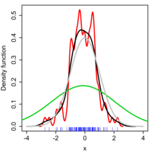
from a sample of 200 points. The figure on the right below shows the true density and two kernel density estimates—one using the rule-of-thumb bandwidth, and the other using a solve-the-equation bandwidth.[7][16] The estimate based on the rule-of-thumb bandwidth is significantly oversmoothed. The Matlab script for this example uses kde.m and is given below.

Comparison between rule of thumb and solve-the-equation bandwidth.

 1 % Data
 2 randn('seed',1)                            % Used for reproducibility
 3 data = [randn(100,1)-10; randn(100,1)+10]; % Two Normals mixed
 4 % True
 5 phi = @(x) exp(-.5*x.^2)/sqrt(2*pi);       % Normal Density
 6 tpdf = @(x) phi(x+10)/2+phi(x-10)/2;       % True Density
 7 % Kernel
 8 h = std(data)*(4/3/numel(data))^(1/5);     % Bandwidth estimated by Silverman's Rule of Thumb
 9 kernel = @(x) mean(phi((x-data)/h)/h);     % Kernel Density
10 kpdf = @(x) arrayfun(kernel,x);            % Elementwise application
11 % Plot
12 figure(2), clf, hold on
13 x = linspace(-25,+25,1000);                % Linear Space
14 plot(x,tpdf(x))                            % Plot True Density
15 plot(x,kpdf(x))                            % Plot Kernel Density with Silverman's Rule of Thumb
16 kde(data)                                  % Plot Kernel Density with Solve-the-Equation Bandwidth

 1 #The same code with R language
 2 #` Data
 3 set.seed(1)                                                     #Used for reproducibility
 4 data = c(rnorm(100,-10,1),rnorm(100,10,1))                      #Two Normals mixed
 5 #` True
 6 phi = function(x) exp(-.5*x^2)/sqrt(2*pi)                       #Normal Density
 7 tpdf = function(x) phi(x+10)/2+phi(x-10)/2                      #True Density
 8 #` Kernel
 9 h = sd(data)*(4/3/length(data))^(1/5)                           #Bandwidth estimated by Silverman's Rule of Thumb
10 Kernel2 = function(x) mean(phi((x-data)/h)/h)                   #Kernel Density
11 kpdf = function(x) sapply(x,Kernel2)                            #Elementwise application
12 #` Plot
13 x=seq(-25,25,length=1000)                                       #Linear Space
14 plot(x,tpdf(x),type="l",ylim=c(0,0.23),col="red")               #Plot True Density
15 par(new=T)
16 plot(x,kpdf(x),type="l",ylim=c(0,0.23),xlab="",ylab="",axes=F)  #Plot Kernel Density with Silverman's Rule of Thumb

Given the sample (x₁, x₂, …, x_n), it is natural to estimate the characteristic function φ(t) = E[e^itX] as

${\displaystyle {\widehat {\varphi }}(t)={\frac {1}{n}}\sum _{j=1}^{n}e^{itx_{j}}}$

Knowing the characteristic function, it is possible to find the corresponding probability density function through the Fourier transform formula. One difficulty with applying this inversion formula is that it leads to a diverging integral, since the estimate ${\displaystyle \scriptstyle {\widehat {\varphi }}(t)}$ is unreliable for large t’s. To circumvent this problem, the estimator ${\displaystyle \scriptstyle {\widehat {\varphi }}(t)}$ is multiplied by a damping function ψ_h(t) = ψ(ht), which is equal to 1 at the origin and then falls to 0 at infinity. The “bandwidth parameter” h controls how fast we try to dampen the function ${\displaystyle \scriptstyle {\widehat {\varphi }}(t)}$. In particular when h is small, then ψ_h(t) will be approximately one for a large range of t’s, which means that ${\displaystyle \scriptstyle {\widehat {\varphi }}(t)}$ remains practically unaltered in the most important region of t’s.

The most common choice for function ψ is either the uniform function ψ(t) = 1{−1 ≤ t ≤ 1}, which effectively means truncating the interval of integration in the inversion formula to [−1/h, 1/h], or the Gaussian function ψ(t) = e^−πt2. Once the function ψ has been chosen, the inversion formula may be applied, and the density estimator will be

${\displaystyle {\begin{aligned}{\widehat {f}}(x)&={\frac {1}{2\pi }}\int _{-\infty }^{+\infty }{\widehat {\varphi }}(t)\psi _{h}(t)e^{-itx}\,dt={\frac {1}{2\pi }}\int _{-\infty }^{+\infty }{\frac {1}{n}}\sum _{j=1}^{n}e^{it(x_{j}-x)}\psi (ht)\,dt\\[5pt]&={\frac {1}{nh}}\sum _{j=1}^{n}{\frac {1}{2\pi }}\int _{-\infty }^{+\infty }e^{-i(ht){\frac {x-x_{j}}{h}}}\psi (ht)\,d(ht)={\frac {1}{nh}}\sum _{j=1}^{n}K{\Big (}{\frac {x-x_{j}}{h}}{\Big )},\end{aligned}}}$

where K is the Fourier transform of the damping function ψ. Thus the kernel density estimator coincides with the characteristic function density estimator.

We can extend the definition of the (global) mode to a local sense and define the local modes:

${\displaystyle M=\{x:g(x)=0,\lambda _{1}(x)<0\}}$

Namely, ${\displaystyle M}$ is the collection of points for which the density function is locally maximized. A natural estimator of ${\displaystyle M}$ is a plug-in from KDE,[23][24] where ${\displaystyle g(x)}$ and ${\displaystyle \lambda _{1}(x)}$ are KDE version of ${\displaystyle g(x)}$ and ${\displaystyle \lambda _{1}(x)}$. Under mild assumptions, ${\displaystyle M_{c}}$ is a consistent estimator of ${\displaystyle M}$. Note that one can use the mean shift algorithm[25][26][27] to compute the estimator ${\displaystyle M_{c}}$ numerically.

A non-exhaustive list of software implementations of kernel density estimators includes:

• In Analytica release 4.4, the Smoothing option for PDF results uses KDE, and from expressions it is available via the built-in Pdf function.
• In C/C++, FIGTree is a library that can be used to compute kernel density estimates using normal kernels. MATLAB interface available.
• In C++, libagf is a library for variable kernel density estimation.
• In C++, mlpack is a library that can compute KDE using many different kernels. It allows to set an error tolerance for faster computation. Python and R interfaces available.
• in C# and F#, Math.NET Numerics is an open source library for numerical computation which includes kernel density estimation
• In CrimeStat, kernel density estimation is implemented using five different kernel functions – normal, uniform, quartic, negative exponential, and triangular. Both single- and dual-kernel density estimate routines are available. Kernel density estimation is also used in interpolating a Head Bang routine, in estimating a two-dimensional Journey-to-crime density function, and in estimating a three-dimensional Bayesian Journey-to-crime estimate.
• In ELKI, kernel density functions can be found in the package de.lmu.ifi.dbs.elki.math.statistics.kernelfunctions
• In ESRI products, kernel density mapping is managed out of the Spatial Analyst toolbox and uses the Quartic(biweight) kernel.
• In Excel, the Royal Society of Chemistry has created an add-in to run kernel density estimation based on their Analytical Methods Committee Technical Brief 4.
• In gnuplot, kernel density estimation is implemented by the smooth kdensity option, the datafile can contain a weight and bandwidth for each point, or the bandwidth can be set automatically[28] according to "Silverman's rule of thumb" (see above).
• In Haskell, kernel density is implemented in the statistics package.
• In IGOR Pro, kernel density estimation is implemented by the StatsKDE operation (added in Igor Pro 7.00). Bandwidth can be user specified or estimated by means of Silverman, Scott or Bowmann and Azzalini. Kernel types are: Epanechnikov, Bi-weight, Tri-weight, Triangular, Gaussian and Rectangular.
• In Java, the Weka (machine learning) package provides weka.estimators.KernelEstimator, among others.
• In JavaScript, the visualization package D3.js offers a KDE package in its science.stats package.
• In JMP, the distribution platform can be used to create univariate kernel density estimates, and the Fit Y by X platform can be used to create bivariate kernel density estimates. It uses the formula ${\displaystyle h=0.9*{\hat {\sigma }}*n^{-0.2}}$, but not the optimized formula mentioned in book of Silverman.
• In Julia, kernel density estimation is implemented in the KernelDensity.jl package.
• In MATLAB, kernel density estimation is implemented through the ksdensity function (Statistics Toolbox). As of the 2018a release of MATLAB, both the bandwidth and kernel smoother can be specified, including other options such as specifying the range of the kernel density Alternatively, a free MATLAB software package which implements an automatic bandwidth selection method[7] is available from the MATLAB Central File Exchange for
  • 1-dimensional data
  • 2-dimensional data
  • n-dimensional data
    A free MATLAB toolbox with implementation of kernel regression, kernel density estimation, kernel estimation of hazard function and many others is available on these pages (this toolbox is a part of the book [29]).
• In Mathematica, numeric kernel density estimation is implemented by the function SmoothKernelDistribution here and symbolic estimation is implemented using the function KernelMixtureDistribution here both of which provide data-driven bandwidths.
• In Minitab, the Royal Society of Chemistry has created a macro to run kernel density estimation based on their Analytical Methods Committee Technical Brief 4.
• In the NAG Library, kernel density estimation is implemented via the g10ba routine (available in both the Fortran[30] and the C[31] versions of the Library).
• In Nuklei, C++ kernel density methods focus on data from the Special Euclidean group ${\displaystyle SE(3)}$.
• In Octave, kernel density estimation is implemented by the kernel_density option (econometrics package).
• In Origin, 2D kernel density plot can be made from its user interface, and two functions, Ksdensity for 1D and Ks2density for 2D can be used from its LabTalk, Python, or C code.
• In Perl, an implementation can be found in the Statistics-KernelEstimation module
• In PHP, an implementation can be found in the MathPHP library
• In Python, many implementations exist: pyqt_fit.kde Module in the PyQt-Fit package, SciPy (scipy.stats.gaussian_kde and scipy.signal.parzen), Statsmodels (KDEUnivariate and KDEMultivariate), and Scikit-learn (KernelDensity) (see comparison[32]). KDEpy supports weighted data and its FFT implementation is orders of magnitude faster than the other implementations. The commonly used pandas library offers support for kde plotting through the plot method (df.plot(kind='kde')). The getdist package for weighted and correlated MCMC samples supports optimized bandwidth, boundary correction and higher-order methods for 1D and 2D distributions. One newly used package for kernel density estimation is seaborn ( import seaborn as sns , sns.kdeplot() ).[33]
• In R, it is implemented through density in the base distribution, and bw.nrd0 function is used in stats package, this function uses the optimized formula in Silverman's book. bkde in the KernSmooth library, ParetoDensityEstimation in the AdaptGauss library (for pareto distribution density estimation), kde in the ks library, dkden and dbckden in the evmix library (latter for boundary corrected kernel density estimation for bounded support), npudens in the np library (numeric and categorical data), sm.density in the sm library. For an implementation of the kde.R function, which does not require installing any packages or libraries, see kde.R. The btb library, dedicated to urban analysis, implements kernel density estimation through kernel_smoothing.
• In SAS, proc kde can be used to estimate univariate and bivariate kernel densities.
• In Apache Spark, you can use the KernelDensity() class (see official documentation for more details )
• In Stata, it is implemented through kdensity;[34] for example histogram x, kdensity. Alternatively a free Stata module KDENS is available from here allowing a user to estimate 1D or 2D density functions.
• In Swift, it is implemented through SwiftStats.KernelDensityEstimation in the open-source statistics library SwiftStats.

Wikimedia Commons has media related to Kernel density estimation.

• Kernel (statistics)
• Kernel smoothing
• Kernel regression
• Density estimation (with presentation of other examples)
• Mean-shift
• Scale space: The triplets {(x, h, KDE with bandwidth h evaluated at x: all x, h > 0} form a scale space representation of the data.
• Multivariate kernel density estimation
• Variable kernel density estimation
• Head/tail breaks

• Introduction to kernel density estimation A short tutorial which motivates kernel density estimators as an improvement over histograms.
• Kernel Bandwidth Optimization A free online tool that instantly generates an optimized kernel density estimate of your data.
• Free Online Software (Calculator) computes the Kernel Density Estimation for any data series according to the following Kernels: Gaussian, Epanechnikov, Rectangular, Triangular, Biweight, Cosine, and Optcosine.
• Kernel Density Estimation Applet An online interactive example of kernel density estimation. Requires .NET 3.0 or later.

References

- Rosenblatt, M. (1956). "Remarks on Some Nonparametric Estimates of a Density Function". The Annals of Mathematical Statistics. 27 (3): 832–837. doi:10.1214/aoms/1177728190.
- Parzen, E. (1962). "On Estimation of a Probability Density Function and Mode". The Annals of Mathematical Statistics. 33 (3): 1065–1076. doi:10.1214/aoms/1177704472. JSTOR 2237880.
- Piryonesi S. Madeh; El-Diraby Tamer E. (2020-06-01). "Role of Data Analytics in Infrastructure Asset Management: Overcoming Data Size and Quality Problems". Journal of Transportation Engineering, Part B: Pavements. 146 (2): 04020022. doi:10.1061/JPEODX.0000175.
- Hastie, Trevor. (2001). The elements of statistical learning : data mining, inference, and prediction : with 200 full-color illustrations. Tibshirani, Robert., Friedman, J. H. (Jerome H.). New York: Springer. ISBN 0-387-95284-5. OCLC 46809224.
- Epanechnikov, V.A. (1969). "Non-parametric estimation of a multivariate probability density". Theory of Probability and Its Applications. 14: 153–158. doi:10.1137/1114019.
- Wand, M.P; Jones, M.C. (1995). Kernel Smoothing. London: Chapman & Hall/CRC. ISBN 978-0-412-55270-0.
- Botev, Z.I.; Grotowski, J.F.; Kroese, D.P. (2010). "Kernel density estimation via diffusion". Annals of Statistics. 38 (5): 2916–2957. arXiv:1011.2602. doi:10.1214/10-AOS799.
- Scott, D. (1979). "On optimal and data-based histograms". Biometrika. 66 (3): 605–610. doi:10.1093/biomet/66.3.605.
- Park, B.U.; Marron, J.S. (1990). "Comparison of data-driven bandwidth selectors". Journal of the American Statistical Association. 85 (409): 66–72. CiteSeerX 10.1.1.154.7321. doi:10.1080/01621459.1990.10475307. JSTOR 2289526.
- Park, B.U.; Turlach, B.A. (1992). "Practical performance of several data driven bandwidth selectors (with discussion)". Computational Statistics. 7: 251–270.
- Cao, R.; Cuevas, A.; Manteiga, W. G. (1994). "A comparative study of several smoothing methods in density estimation". Computational Statistics and Data Analysis. 17 (2): 153–176. doi:10.1016/0167-9473(92)00066-Z.
- Jones, M.C.; Marron, J.S.; Sheather, S. J. (1996). "A brief survey of bandwidth selection for density estimation". Journal of the American Statistical Association. 91 (433): 401–407. doi:10.2307/2291420. JSTOR 2291420.
- Sheather, S.J. (1992). "The performance of six popular bandwidth selection methods on some real data sets (with discussion)". Computational Statistics. 7: 225–250, 271–281.
- Agarwal, N.; Aluru, N.R. (2010). "A data-driven stochastic collocation approach for uncertainty quantification in MEMS" (PDF). International Journal for Numerical Methods in Engineering. 83 (5): 575–597.
- Xu, X.; Yan, Z.; Xu, S. (2015). "Estimating wind speed probability distribution by diffusion-based kernel density method". Electric Power Systems Research. 121: 28–37. doi:10.1016/j.epsr.2014.11.029.
- Sheather, S.J.; Jones, M.C. (1991). "A reliable data-based bandwidth selection method for kernel density estimation". Journal of the Royal Statistical Society, Series B. 53 (3): 683–690. doi:10.1111/j.2517-6161.1991.tb01857.x. JSTOR 2345597.
- Rudemo, M. (1982). "Empirical choice of histograms and kernel density estimators". Scandinavian Journal of Statistics. 9 (2): 65–78. JSTOR 4615859.
- Bowman, A.W. (1984). "An alternative method of cross-validation for the smoothing of density estimates". Biometrika. 71 (2): 353–360. doi:10.1093/biomet/71.2.353.
- Hall, P.; Marron, J.S.; Park, B.U. (1992). "Smoothed cross-validation". Probability Theory and Related Fields. 92: 1–20. doi:10.1007/BF01205233.
- Wahba, G. (1975). "Optimal convergence properties of variable knot, kernel, and orthogonal series methods for density estimation". Annals of Statistics. 3 (1): 15–29. doi:10.1214/aos/1176342997.
- Buch-Larsen, TINE (2005). "Kernel density estimation for heavy-tailed distributions using the Champernowne transformation". Statistics. 39 (6): 503–518. CiteSeerX 10.1.1.457.1544. doi:10.1080/02331880500439782.
- Silverman, B.W. (1986). Density Estimation for Statistics and Data Analysis. London: Chapman & Hall/CRC. p. 45. ISBN 978-0-412-24620-3.
- Chen, Yen-Chi; Genovese, Christopher R.; Wasserman, Larry (2016). "A comprehensive approach to mode clustering". Electronic Journal of Statistics. 10 (1): 210–241. doi:10.1214/15-ejs1102. ISSN 1935-7524.
- Chazal, Frédéric; Fasy, Brittany Terese; Lecci, Fabrizio; Rinaldo, Alessandro; Wasserman, Larry (2014). "Stochastic Convergence of Persistence Landscapes and Silhouettes". Annual Symposium on Computational Geometry - SOCG'14. New York, New York, USA: ACM Press: 474–483. doi:10.1145/2582112.2582128. ISBN 978-1-4503-2594-3.
- Fukunaga, K.; Hostetler, L. (January 1975). "The estimation of the gradient of a density function, with applications in pattern recognition". IEEE Transactions on Information Theory. 21 (1): 32–40. doi:10.1109/tit.1975.1055330. ISSN 0018-9448.
- Yizong Cheng (1995). "Mean shift, mode seeking, and clustering". IEEE Transactions on Pattern Analysis and Machine Intelligence. 17 (8): 790–799. doi:10.1109/34.400568. ISSN 0162-8828.
- Comaniciu, D.; Meer, P. (May 2002). "Mean shift: a robust approach toward feature space analysis". IEEE Transactions on Pattern Analysis and Machine Intelligence. 24 (5): 603–619. doi:10.1109/34.1000236. ISSN 0162-8828.
- Janert, Philipp K (2009). Gnuplot in action : understanding data with graphs. Connecticut, USA: Manning Publications. ISBN 978-1-933988-39-9. See section 13.2.2 entitled Kernel density estimates.
- Horová, I.; Koláček, J.; Zelinka, J. (2012). Kernel Smoothing in MATLAB: Theory and Practice of Kernel Smoothing. Singapore: World Scientific Publishing. ISBN 978-981-4405-48-5.
- The Numerical Algorithms Group. "NAG Library Routine Document: nagf_smooth_kerndens_gauss (g10baf)" (PDF). NAG Library Manual, Mark 23. Retrieved 2012-02-16.
- The Numerical Algorithms Group. "NAG Library Routine Document: nag_kernel_density_estim (g10bac)" (PDF). NAG Library Manual, Mark 9. Archived from the original (PDF) on 2011-11-24. Retrieved 2012-02-16.
- Vanderplas, Jake (2013-12-01). "Kernel Density Estimation in Python". Retrieved 2014-03-12.
- "seaborn.kdeplot — seaborn 0.10.1 documentation". seaborn.pydata.org. Retrieved 2020-05-12.
- https://www.stata.com/manuals15/rkdensity.pdf
External links