Bose–Einstein statistics
In quantum statistics, Bose–Einstein (B–E) statistics describe one of two possible ways in which a collection of non-interacting, indistinguishable particles may occupy a set of available discrete energy states at thermodynamic equilibrium. The aggregation of particles in the same state, which is a characteristic of particles obeying Bose–Einstein statistics, accounts for the cohesive streaming of laser light and the frictionless creeping of superfluid helium. The theory of this behaviour was developed (1924–25) by Satyendra Nath Bose, who recognized that a collection of identical and indistinguishable particles can be distributed in this way. The idea was later adopted and extended by Albert Einstein in collaboration with Bose.
| Statistical mechanics |
|---|
 |
The Bose–Einstein statistics apply only to those particles not limited to single occupancy of the same state—that is, particles that do not obey the Pauli exclusion principle restrictions. Such particles have integer values of spin and are named bosons, after the statistics that correctly describe their behaviour. There must also be no significant interaction between the particles.

Bose–Einstein distribution
At low temperatures, bosons behave differently from fermions (which obey the Fermi–Dirac statistics) in a way that an unlimited number of them can "condense" into the same energy state. This apparently unusual property also gives rise to the special state of matter – the Bose–Einstein condensate. Fermi–Dirac and Bose–Einstein statistics apply when quantum effects are important and the particles are "indistinguishable". Quantum effects appear if the concentration of particles satisfies

where N is the number of particles, V is the volume, and nq is the quantum concentration, for which the interparticle distance is equal to the thermal de Broglie wavelength, so that the wavefunctions of the particles are barely overlapping.
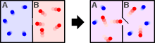
Fermi–Dirac statistics apply to fermions (particles that obey the Pauli exclusion principle), and Bose–Einstein statistics apply to bosons. As the quantum concentration depends on temperature, most systems at high temperatures obey the classical (Maxwell–Boltzmann) limit, unless they also have a very high density, as for a white dwarf. Both Fermi–Dirac and Bose–Einstein become Maxwell–Boltzmann statistics at high temperature or at low concentration.
B–E statistics was introduced for photons in 1924 by Bose and generalized to atoms by Einstein in 1924–25.
The expected number of particles in an energy state i for B–E statistics is:

with εi > μ and where ni is the number of particles in state i over total number of particles of all energy states. gi is the degeneracy of energy level i, εi is the energy of the i-th state, μ is the chemical potential, kB is the Boltzmann constant, and T is absolute temperature.
For comparison, the average number of fermions with energy given by Fermi–Dirac particle-energy distribution has a similar form:


As mentioned above, both the Bose–Einstein distribution and the Fermi–Dirac distribution approaches the Maxwell–Boltzmann distribution in the limit of high temperature and low particle density, without the need for any ad hoc assumptions:
- In the limit of low particle density, , therefore or equivalently . In that case, , which is the result from Maxwell-Boltzmann statistics.
- In the limit of high temperature, the particles are distributed over a large range of energy values, therefore the occupancy on each state (especially the high energy ones with ) is again very small, . This again reduces to Maxwell-Boltzmann statistics.


In addition to reducing to the Maxwell–Boltzmann distribution in the limit of high and low density, B–E statistics also reduce to Rayleigh–Jeans law distribution for low energy states with
, namely


History
While presenting a lecture at the University of Dhaka (in what was then British India and now Bangladesh) on the theory of radiation and the ultraviolet catastrophe, Satyendra Nath Bose intended to show his students that the contemporary theory was inadequate, because it predicted results not in accordance with experimental results. During this lecture, Bose committed an error in applying the theory, which unexpectedly gave a prediction that agreed with the experiment. The error was a simple mistake—similar to arguing that flipping two fair coins will produce two heads one-third of the time—that would appear obviously wrong to anyone with a basic understanding of statistics (remarkably, this error resembled the famous blunder by d'Alembert known from his Croix ou Pile article[1][2]). However, the results it predicted agreed with experiment, and Bose realized it might not be a mistake after all. For the first time, he took the position that the Maxwell–Boltzmann distribution would not be true for all microscopic particles at all scales. Thus, he studied the probability of finding particles in various states in phase space, where each state is a little patch having phase volume of h3, and the position and momentum of the particles are not kept particularly separate but are considered as one variable.
Bose adapted this lecture into a short article called Planck's Law and the Hypothesis of Light Quanta[3][4] and submitted it to the Philosophical Magazine. However, the referee's report was negative, and the paper was rejected. Undaunted, he sent the manuscript to Albert Einstein requesting publication in the Zeitschrift für Physik. Einstein immediately agreed, personally translated the article from English into German (Bose had earlier translated Einstein's article on the theory of General Relativity from German to English), and saw to it that it was published. Bose's theory achieved respect when Einstein sent his own paper in support of Bose's to Zeitschrift für Physik, asking that they be published together. The paper came out in 1924.[5]
The reason Bose produced accurate results was that since photons are indistinguishable from each other, one cannot treat any two photons having equal energy as being two distinct identifiable photons. By analogy, if in an alternate universe coins were to behave like photons and other bosons, the probability of producing two heads would indeed be one-third, and so is the probability of getting a head and a tail which equals one-half for the conventional (classical, distinguishable) coins. Bose's "error" leads to what is now called Bose–Einstein statistics.
Bose and Einstein extended the idea to atoms and this led to the prediction of the existence of phenomena which became known as Bose–Einstein condensate, a dense collection of bosons (which are particles with integer spin, named after Bose), which was demonstrated to exist by experiment in 1995.
Derivation
Derivation from the microcanonical ensemble
In the microcanonical ensemble, one considers a system with fixed energy, volume, and number of particles. We take a system composed of identical bosons, of which have energy and are distributed over levels or states with the same energy , i.e. is the degeneracy associated with energy of total energy . Calculation of the number of arrangements of particles distributed among states is a problem of combinatorics. Since particles and states are indistinguishable in the quantum mechanical context here, and starting with a state, the number of arrangements is


where is the k-combination of a set with m elements.

If we start with a particle first, the number is

The sum is

Since here all numbers are large, the distinction is irrelevant in the present context. The total number of arrangements in an ensemble of bosons is

The maximum number of arrangements determining the corresponding occupation number is obtained looking the condition that maximizes the entropy, or equivalently, setting and taking the subsidiary conditions into account (as Lagrange multipliers).[6] The result for a large number of particles is the Bose–Einstein distribution.


The expressions are of considerable interest in many problems of combinatorics. For non-huge values of and the binomial coefficients are given by Pascal's triangles. For more details about the combinatorics, see the notes of the canonical derivation.


Derivation from the grand canonical ensemble
The Bose–Einstein distribution, which applies only to a quantum system of non-interacting bosons, is naturally derived from the grand canonical ensemble without any approximations.[7] In this ensemble, the system is able to exchange energy and exchange particles with a reservoir (temperature T and chemical potential µ fixed by the reservoir).
Due to the non-interacting quality, each available single-particle level (with energy level ϵ) forms a separate thermodynamic system in contact with the reservoir. That is, the number of particles within the overall system that occupy a given single particle state form a sub-ensemble that is also grand canonical ensemble; hence, it may be analysed through the construction of a grand partition function.
Every single-particle state is of a fixed energy, . As the sub-ensemble associated with a single-particle state varies by the number of particles only, it is clear that the total energy of the sub-ensemble is also directly proportional to the number of particles in the single-particle state; where is the number of particles, the total energy of the sub-ensemble will then be . Beginning with the standard expression for a grand partition function and replacing with , the grand partition function takes the form


This formula applies to fermionic systems as well as bosonic systems. Fermi-Dirac statistics arise when considering the effect of the Pauli exclusion principle: whilst the number of fermions occupying the same single-particle state can only be either 1 or 0, the number of bosons occupying a single particle state may be any integer. Thus, the grand partition function for bosons can be considered a geometric series and may be evaluated as such:

and the average particle number for that single-particle substate is given by

This result applies for each single-particle level and thus forms the Bose–Einstein distribution for the entire state of the system.[8][9]
The variance in particle number (due to thermal fluctuations) may also be derived, the result can be expressed in terms of the value just derived:


As a result, for highly occupied states the standard deviation of the particle number of an energy level is very large, slightly larger than the particle number itself: . This large uncertainty is due to the fact that the probability distribution for the number of bosons in a given energy level is a geometric distribution; somewhat counterintuitively, the most probable value for N is always 0. (In contrast, classical particles have instead a Poisson distribution in particle number for a given state, with a much smaller uncertainty of , and with the most-probable N value being near .)


Derivation in the canonical approach
It is also possible to derive approximate Bose–Einstein statistics in the canonical ensemble. These derivations are lengthy and only yield the above results in the asymptotic limit of a large number of particles. The reason is that the total number of bosons is fixed in the canonical ensemble. The Bose–Einstein distribution in this case can be derived as in most texts by maximization, but the mathematically best derivation is by the Darwin–Fowler method of mean values as emphasized by Dingle.[10] See also Müller-Kirsten.[6] The fluctuations of the ground state in the condensed region are however markedly different in the canonical and grand-canonical ensembles.[11]
Suppose we have a number of energy levels, labeled by index , each level having energy and containing a total of particles. Suppose each level contains distinct sublevels, all of which have the same energy, and which are distinguishable. For example, two particles may have different momenta, in which case they are distinguishable from each other, yet they can still have the same energy. The value of associated with level is called the "degeneracy" of that energy level. Any number of bosons can occupy the same sublevel.


Let be the number of ways of distributing particles among the sublevels of an energy level. There is only one way of distributing particles with one sublevel, therefore . It is easy to see that there are ways of distributing particles in two sublevels which we will write as:


With a little thought (see Notes below) it can be seen that the number of ways of distributing particles in three sublevels is

so that

where we have used the following theorem involving binomial coefficients:

Continuing this process, we can see that is just a binomial coefficient (See Notes below)

For example, the population numbers for two particles in three sublevels are 200, 110, 101, 020, 011, or 002 for a total of six which equals 4!/(2!2!). The number of ways that a set of occupation numbers can be realized is the product of the ways that each individual energy level can be populated:

where the approximation assumes that .

Following the same procedure used in deriving the Maxwell–Boltzmann statistics, we wish to find the set of for which W is maximised, subject to the constraint that there be a fixed total number of particles, and a fixed total energy. The maxima of and occur at the same value of and, since it is easier to accomplish mathematically, we will maximise the latter function instead. We constrain our solution using Lagrange multipliers forming the function:


Using the approximation and using Stirling's approximation for the factorials gives


Where K is the sum of a number of terms which are not functions of the . Taking the derivative with respect to , and setting the result to zero and solving for , yields the Bose–Einstein population numbers:

By a process similar to that outlined in the Maxwell–Boltzmann statistics article, it can be seen that:

which, using Boltzmann's famous relationship becomes a statement of the second law of thermodynamics at constant volume, and it follows that and where S is the entropy, is the chemical potential, kB is Boltzmann's constant and T is the temperature, so that finally:


Note that the above formula is sometimes written:

where is the absolute activity, as noted by McQuarrie.[12]

Also note that when the particle numbers are not conserved, removing the conservation of particle numbers constraint is equivalent to setting and therefore the chemical potential to zero. This will be the case for photons and massive particles in mutual equilibrium and the resulting distribution will be the Planck distribution.

A much simpler way to think of Bose–Einstein distribution function is to consider that n particles are denoted by identical balls and g shells are marked by g-1 line partitions. It is clear that the permutations of these n balls and g − 1 partitions will give different ways of arranging bosons in different energy levels. Say, for 3 (= n) particles and 3 (= g) shells, therefore (g − 1) = 2, the arrangement might be |●●|●, or ||●●●, or |●|●● , etc. Hence the number of distinct permutations of n + (g-1) objects which have n identical items and (g − 1) identical items will be:

OR
The purpose of these notes is to clarify some aspects of the derivation of the Bose–Einstein (B–E) distribution for beginners. The enumeration of cases (or ways) in the B–E distribution can be recast as follows. Consider a game of dice throwing in which there are dice, with each die taking values in the set , for . The constraints of the game are that the value of a die , denoted by , has to be greater than or equal to the value of die , denoted by , in the previous throw, i.e., . Thus a valid sequence of die throws can be described by an n-tuple , such that . Let denote the set of these valid n-tuples:


(1)

Then the quantity (defined above as the number of ways to distribute particles among the sublevels of an energy level) is the cardinality of , i.e., the number of elements (or valid n-tuples) in . Thus the problem of finding an expression for becomes the problem of counting the elements in .
Example n = 4, g = 3:
-
- (there are elements in )


Subset is obtained by fixing all indices to , except for the last index, , which is incremented from to . Subset is obtained by fixing , and incrementing from to . Due to the constraint on the indices in , the index must automatically take values in . The construction of subsets and follows in the same manner.


Each element of can be thought of as a multiset of cardinality ; the elements of such multiset are taken from the set of cardinality , and the number of such multisets is the multiset coefficient


More generally, each element of is a multiset of cardinality (number of dice) with elements taken from the set of cardinality (number of possible values of each die), and the number of such multisets, i.e., is the multiset coefficient

(2)

which is exactly the same as the formula for , as derived above with the aid of a theorem involving binomial coefficients, namely
(3)
To understand the decomposition
(4)

or for example, and

let us rearrange the elements of as follows


Clearly, the subset of is the same as the set

- .

By deleting the index (shown in red with double underline) in the subset of , one obtains the set


- .

In other words, there is a one-to-one correspondence between the subset of and the set . We write

- .

Similarly, it is easy to see that
- (empty set).


Thus we can write

or more generally,
;
(5)

and since the sets

are non-intersecting, we thus have
,
(6)

with the convention that
(7)

Continuing the process, we arrive at the following formula

Using the convention (7)2 above, we obtain the formula
(8)

keeping in mind that for and being constants, we have


.
(9)

It can then be verified that (8) and (2) give the same result for , , , etc.


Interdisciplinary applications
Viewed as a pure probability distribution, the Bose–Einstein distribution has found application in other fields:
- In recent years, Bose Einstein statistics have also been used as a method for term weighting in information retrieval. The method is one of a collection of DFR ("Divergence From Randomness") models,[13] the basic notion being that Bose Einstein statistics may be a useful indicator in cases where a particular term and a particular document have a significant relationship that would not have occurred purely by chance. Source code for implementing this model is available from the Terrier project at the University of Glasgow.
- The evolution of many complex systems, including the World Wide Web, business, and citation networks, is encoded in the dynamic web describing the interactions between the system's constituents. Despite their irreversible and nonequilibrium nature these networks follow Bose statistics and can undergo Bose–Einstein condensation. Addressing the dynamical properties of these nonequilibrium systems within the framework of equilibrium quantum gases predicts that the "first-mover-advantage," "fit-get-rich(FGR)," and "winner-takes-all" phenomena observed in competitive systems are thermodynamically distinct phases of the underlying evolving networks.[14]
See also
- Bose–Einstein correlations
- Bose–Einstein condensate
- Bose gas
- Einstein solid
- Higgs boson
- Parastatistics
- Planck's law of black body radiation
- Superconductivity
- Fermi–Dirac statistics
- Maxwell–Boltzmann statistics
Notes
- d'Alembert, Jean (1754). "Croix ou pile". L'Encyclopédie (in French). 4.
- d'Alembert, Jean (1754). "CROIX OU PILE" [Translated by Richard J. Pulskamp] (PDF). Xavier University. Retrieved 2019-01-14.
- See p. 14, note 3, of the thesis: Michelangeli, Alessandro (October 2007). Bose–Einstein condensation: Analysis of problems and rigorous results (PDF) (Ph.D.). International School for Advanced Studies. Archived (PDF) from the original on 3 November 2018. Retrieved 14 February 2019. Lay summary.
- Bose (2 July 1924). "Planck's law and the hypothesis of light quanta" (PostScript). University of Oldenburg. Retrieved 30 November 2016.
- Bose (1924), "Plancks Gesetz und Lichtquantenhypothese", Zeitschrift für Physik (in German), 26 (1): 178–181, Bibcode:1924ZPhy...26..178B, doi:10.1007/BF01327326
- H.J.W. Müller-Kirsten, Basics of Statistical Physics, 2nd ed., World Scientific (2013), ISBN 978-981-4449-53-3.
- Srivastava, R. K.; Ashok, J. (2005). "Chapter 7". Statistical Mechanics. New Delhi: PHI Learning Pvt. Ltd. ISBN 9788120327825.
- "Chapter 6". Statistical Mechanics. January 2005. ISBN 9788120327825.
- The BE distribution can be derived also from thermal field theory.
- R.B. Dingle, Asymptotic Expansions: Their Derivation and Interpretation, Academic Press (1973), pp. 267–271.
- Ziff R. M; Kac, M.; Uhlenbeck, G. E. (1977). "The ideal Bose–Einstein gas, revisited." Phys. Reports 32: 169-248.
- See McQuarrie in citations
- Amati, G.; C. J. Van Rijsbergen (2002). "Probabilistic models of information retrieval based on measuring the divergence from randomness " ACM TOIS 20(4):357–389.
- Bianconi, G.; Barabási, A.-L. (2001). "Bose–Einstein Condensation in Complex Networks." Phys. Rev. Lett. 86: 5632–35.
References
- Annett, James F. (2004). Superconductivity, Superfluids and Condensates. New York: Oxford University Press. ISBN 0-19-850755-0.
- Carter, Ashley H. (2001). Classical and Statistical Thermodynamics. Upper Saddle River, New Jersey: Prentice Hall. ISBN 0-13-779208-5.
- Griffiths, David J. (2005). Introduction to Quantum Mechanics (2nd ed.). Upper Saddle River, New Jersey: Pearson, Prentice Hall. ISBN 0-13-191175-9.
- McQuarrie, Donald A. (2000). Statistical Mechanics (1st ed.). Sausalito, California 94965: University Science Books. p. 55. ISBN 1-891389-15-7.CS1 maint: location (link)
| Theory | ||
|---|---|---|
| Statistical thermodynamics | ||
| Models | ||
| Mathematical approaches | ||
| Critical phenomena |
| |
| Entropy |
| |
| Applications | ||