Microcanonical ensemble
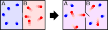
In statistical mechanics, a micro-canonical ensemble is the statistical ensemble that is used to represent the possible states of a mechanical system that has an exactly specified total energy.[1] The system is assumed to be isolated in the sense that the system cannot exchange energy or particles with its environment, so that (by conservation of energy) the energy of the system remains exactly the same as time goes on. The system's energy, composition, volume, and shape are kept the same in all possible states of the system.
| Statistical mechanics |
|---|
 |
The macroscopic variables of the micro-canonical ensemble are quantities that influence the nature of the system's micro-states such as the total number of particles in the system (symbol: N), the system's volume (symbol: V), as well as the total energy in the system (symbol: E). This ensemble is therefore sometimes called the NVE ensemble, as each of these three quantities is a constant of the ensemble.
In simple terms, the micro-canonical ensemble is defined by assigning an equal probability to every micro-state whose energy falls within a range centered at E. All other micro-states are given a probability of zero. Since the probabilities must add up to 1, the probability P is the inverse of the number of micro-states W within the range of energy,

The range of energy is then reduced in width until it is infinitesimally narrow, still centered at E. In the limit of this process, the micro-canonical ensemble is obtained.[1]
Applicability
The micro-canonical ensemble is sometimes considered to be the fundamental distribution of statistical thermodynamics, as its form can be justified on elementary grounds such as the principle of indifference: the micro-canonical ensemble describes the possible states of an isolated mechanical system when the energy is known exactly, but without any more information about the internal state. Also, in some special systems the evolution is ergodic in which case the micro-canonical ensemble is equal to the time-ensemble when starting out with a single state of energy E (a time-ensemble is the ensemble formed of all future states evolved from a single initial state).
In practice, the micro-canonical ensemble does not correspond to an experimentally realistic situation. With a real physical system there is at least some uncertainty in energy, due to uncontrolled factors in the preparation of the system. Besides the difficulty of finding an experimental analogue, it is difficult to carry out calculations that satisfy exactly the requirement of fixed energy since it prevents logically independent parts of the system from being analyzed separately. Moreover, there are ambiguities regarding the appropriate definitions of quantities such as entropy and temperature in the micro-canonical ensemble.[1]
Systems in thermal equilibrium with their environment have uncertainty in energy, and are instead described by the canonical ensemble or the grand canonical ensemble, the latter if the system is also in equilibrium with its environment in respect to particle exchange.
Properties
- Statistical equilibrium (steady state): A microcanonical ensemble does not evolve over time, despite the fact that every constituent of the ensemble is in motion. This is because the ensemble is defined strictly as a function of a conserved quantity of the system (energy).[1]
- Maximal information entropy: For a given mechanical system (fixed N, V) and a given range of energy, the uniform distribution of probability over microstates (as in the microcanonical ensemble) maximizes the ensemble average −⟨log P⟩.[1]
- Three different quantities called "entropy" can be defined for the microcanonical ensemble.[2] Each can be defined in terms of the phase volume function v(E), which counts the total number of states with energy less than E (see the Precise expressions section for the mathematical definition of v):
- the Boltzmann entropy[note 1]
- the volume entropy
- the surface entropy
- the Boltzmann entropy[note 1]
- Different "temperatures" may be defined by differentiating the entropy quantities [3]:
- Microcanonical pressure may be defined :
- Microcanonical chemical potential may be defined :


Thermodynamic analogies
Early work in statistical mechanics by Ludwig Boltzmann led to his eponymous entropy equation for a system of a given total energy, S = k log W, where W is the number of distinct states accessible by the system at that energy. Boltzmann did not elaborate too deeply on what exactly constitutes the set of distinct states of a system, besides the special case of an ideal gas. This topic was investigated to completion by Josiah Willard Gibbs who developed the generalized statistical mechanics for arbitrary mechanical systems, and defined the micro-canonical ensemble described in this article.[1] Gibbs investigated carefully the analogies between the micro-canonical ensemble and thermodynamics, especially how they break down in the case of systems of few degrees of freedom. He introduced two further definitions of micro-canonical entropy that do not depend on ω - the volume and surface entropy described above. (Note that the surface entropy differs from the Boltzmann entropy only by an ω-dependent offset.)
The volume entropy Sv and associated Tv form a close analogy to thermodynamic entropy and temperature. It is possible to show exactly that

(⟨P⟩ is the ensemble average pressure) as expected for the first law of thermodynamics. A similar equation can be found for the surface (Boltzmann) entropy and its associated Ts, however the "pressure" in this equation is a complicated quantity unrelated to the average pressure.[1]
The micro-canonical Tv and Ts are not entirely satisfactory in their analogy to temperature. Outside of the thermodynamic limit, a number of artifacts occur.
- Nontrivial result of combining two systems: Two systems, each described by an independent micro-canonical ensemble, can be brought into thermal contact and be allowed to equilibriate into a combined system also described by a micro-canonical ensemble. Unfortunately, the energy flow between the two systems cannot be predicted based on the initial T's. Even when the initial T's are equal, there may be energy transferred. Moreover, the T of the combination is different from the initial values. This contradicts the intuition that temperature should be an intensive quantity, and that two equal-temperature systems should be unaffected by being brought into thermal contact.[1]
- Strange behavior for few-particle systems: Many results such as the micro-canonical Equipartition theorem acquire a one- or two-degree of freedom offset when written in terms of Ts. For a small systems this offset is significant, and so if we make Ss the analogue of entropy, several exceptions need to be made for systems with only one or two degrees of freedom.[1]
- Spurious negative temperatures: A negative Ts occurs whenever the density of states is decreasing with energy. In some systems the density of states is not monotonic in energy, and so Ts can change sign multiple times as the energy is increased.[4][5]
The preferred solution to these problems is avoid use of the micro-canonical ensemble. In many realistic cases a system is thermostatted to a heat bath so that the energy is not precisely known. Then, a more accurate description is the canonical ensemble or grand canonical ensemble, both of which have complete correspondence to thermodynamics.[6]
Precise expressions for the ensemble
The precise mathematical expression for a statistical ensemble depends on the kind of mechanics under consideration—quantum or classical—since the notion of a "micro-state" is considerably different in these two cases. In quantum mechanics, diagonalization provides a discrete set of micro-states with specific energies. The classical mechanical case involves instead an integral over canonical phase space, and the size of micro-states in phase space can be chosen somewhat arbitrarily.
To construct the micro-canonical ensemble, it is necessary in both types of mechanics to first specify a range of energy. In the expressions below the function (a function of H, peaking at E with width ω) will be used to represent the range of energy in which to include states. An example of this function would be[1]


or, more smoothly,

Quantum mechanical
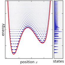
A statistical ensemble in quantum mechanics is represented by a density matrix, denoted by . The micro-canonical ensemble can be written using bra–ket notation, in terms of the system's energy eigenstates and energy eigenvalues. Given a complete basis of energy eigenstates |ψi⟩, indexed by i, the micro-canonical ensemble is


where the Hi are the energy eigenvalues determined by (here Ĥ is the system's total energy operator, i. e., Hamiltonian operator). The value of W is determined by demanding that is a normalized density matrix, and so


The state volume function (used to calculate entropy) is given by

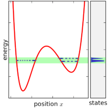
The micro-canonical ensemble is defined by taking the limit of the density matrix as the energy width goes to zero, however a problematic situation occurs once the energy width becomes smaller than the spacing between energy levels. For very small energy width, the ensemble does not exist at all for most values of E, since no states fall within the range. When the ensemble does exist, it typically only contains one (or two) states, since in a complex system the energy levels are only ever equal by accident (see random matrix theory for more discussion on this point). Moreover, the state-volume function also increases only in discrete increments, and so its derivative is only ever infinite or zero, making it difficult to define the density of states. This problem can be solved by not taking the energy range completely to zero and smoothing the state-volume function, however this makes the definition of the ensemble more complicated, since it becomes then necessary to specify the energy range in addition to other variables (together, an NVEω ensemble).
Classical mechanical
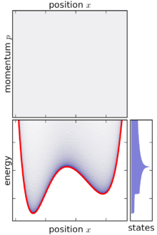

In classical mechanics, an ensemble is represented by a joint probability density function ρ(p1, … pn, q1, … qn) defined over the system's phase space.[1] The phase space has n generalized coordinates called q1, … qn, and n associated canonical momenta called p1, … pn.
The probability density function for the micro-canonical ensemble is:

where
- H is the total energy (Hamiltonian) of the system, a function of the phase (p1, … qn),
- h is an arbitrary but predetermined constant with the units of energy×time, setting the extent of one micro-state and providing correct dimensions to ρ.[note 2]
- C is an overcounting correction factor, often used for particle systems where identical particles are able to change place with each other.[note 3]
Again, the value of W is determined by demanding that ρ is a normalized probability density function:

This integral is taken over the entire phase space. The state volume function (used to calculate entropy) is defined by

As the energy width ω is taken to zero, the value of W decreases in proportion to ω as W = ω (dv/dE).
Based on the above definition, the micro-canonical ensemble can be visualized as an infinitesimally thin shell in phase space, centered on a constant-energy surface. Although the micro-canonical ensemble is confined to this surface, it is not necessarily uniformly distributed over that surface: if the gradient of energy in phase space varies, then the micro-canonical ensemble is "thicker" (more concentrated) in some parts of the surface than others. This feature is an unavoidable consequence of requiring that the micro-canonical ensemble is a steady-state ensemble.
Perfect Gas Entropy and thermodynamic limit
Let's use the microcanonical description for characterize a perfect gas composed of N punctual particles in a volume V, of masse m and a void spin. The isolated gas has a total energy . As a reminder, the energy of a particule is quantified : . First of all, we should determine the number of vector having a norm such as while respecting the discretization of .


Thus the phase volume function v(E) could be considered as the number of elementary mesh that we could put in a sphere of radius . For N particles gas, k dimension is equal to 3N, the elementary mesh is then a hypercube of volume and the (3N-hyper) sphere of radius has a volume of , where is the gamma function.


Hence,

In order to determine the entropy we must exprimed

Particles being indistinguishable we divide the number of possible state by N! as part of Maxwell-Boltzmann approximation.
The entropy is then egal to : ,where we used Stirling's approximation with , finally we find the Sackur–Tetrode equation.


We find easily the microcanonical temperatures , we find the well known result of Kinetic theory of gases.

Moreover we find the famous ideal gas law, indeed we have

Notes
- SB is the information entropy, or Gibbs entropy, for the specific case of the microcanonical ensemble. Note that it depends on the energy width ω.
- (Historical note) Gibbs' original ensemble effectively set h = 1 [energy unit]×[time unit], leading to unit-dependence in the values of some thermodynamic quantities like entropy and chemical potential. Since the advent of quantum mechanics, h is often taken to be equal to Planck's constant in order to obtain a semiclassical correspondence with quantum mechanics.
- In a system of N identical particles, C = N! (factorial of N). This factor corrects the overcounting in phase space due to identical physical states being found in multiple locations. See the statistical ensemble article for more information on this overcounting.
References
- Gibbs, Josiah Willard (1902). Elementary Principles in Statistical Mechanics. New York: Charles Scribner's Sons.
- Huang, Kerson (1987). Statistical Mechanics. Wiley. p. 134. ISBN 978-0471815181.
- "The Microcanonical Ensemble". chem.libretexts. Retrieved May 3, 2020.
- Jörn Dunkel; Stefan Hilbert (2013). "Inconsistent thermostatistics and negative absolute temperatures". Nature Physics. 10 (1): 67–72. arXiv:1304.2066. Bibcode:2014NatPh..10...67D. doi:10.1038/nphys2815.
- See further references at https://sites.google.com/site/entropysurfaceorvolume/
- Tolman, R. C. (1938). The Principles of Statistical Mechanics. Oxford University Press.
| Theory | ||
|---|---|---|
| Statistical thermodynamics | ||
| Models | ||
| Mathematical approaches | ||
| Critical phenomena |
| |
| Entropy |
| |
| Applications | ||