Modularity (networks)

Many scientifically important problems can be represented and empirically studied using networks. For example, biological and social patterns, the World Wide Web, metabolic networks, food webs, neural networks and pathological networks are real world problems that can be mathematically represented and topologically studied to reveal some unexpected structural features.[1] Most of these networks possess a certain community structure that has substantial importance in building an understanding regarding the dynamics of the network. For instance, a closely connected social community will imply a faster rate of transmission of information or rumor among them than a loosely connected community. Thus, if a network is represented by a number of individual nodes connected by links which signify a certain degree of interaction between the nodes, communities are defined as groups of densely interconnected nodes that are only sparsely connected with the rest of the network. Hence, it may be imperative to identify the communities in networks since the communities may have quite different properties such as node degree, clustering coefficient, betweenness, centrality.[2] etc., from that of the average network. Modularity is one such measure, which when maximized, leads to the appearance of communities in a given network.

Modularity is the fraction of the edges that fall within the given groups minus the expected fraction if edges were distributed at random. The value of the modularity for unweighted and undirected graphs lies in the range ${\displaystyle [-1/2,1]}$.[3] It is positive if the number of edges within groups exceeds the number expected on the basis of chance. For a given division of the network's vertices into some modules, modularity reflects the concentration of edges within modules compared with random distribution of links between all nodes regardless of modules.

There are different methods for calculating modularity.[1] In the most common version of the concept, the randomization of the edges is done so as to preserve the degree of each vertex. Consider a graph with ${\displaystyle n}$ nodes and ${\displaystyle m}$ links (edges) such that the graph can be partitioned into two communities using a membership variable ${\displaystyle s}$. If a node ${\displaystyle v}$ belongs to community 1, ${\displaystyle s_{v}=1}$, or if ${\displaystyle v}$ belongs to community 2, ${\displaystyle s_{v}=-1}$. Let the adjacency matrix for the network be represented by ${\displaystyle A}$, where ${\displaystyle A_{vw}=0}$ means there's no edge (no interaction) between nodes ${\displaystyle v}$ and ${\displaystyle w}$ and ${\displaystyle A_{vw}=1}$ means there is an edge between the two. Also for simplicity we consider an undirected network. Thus ${\displaystyle A_{vw}=A_{wv}}$. (It is important to note that multiple edges may exist between two nodes, but here we assess the simplest case).

Modularity ${\displaystyle Q}$ is then defined as the fraction of edges that fall within group 1 or 2, minus the expected number of edges within groups 1 and 2 for a random graph with the same node degree distribution as the given network.

The expected number of edges shall be computed using the concept of a configuration model.[4] The configuration model is a randomized realization of a particular network. Given a network with ${\displaystyle n}$ nodes, where each node ${\displaystyle v}$ has a node degree ${\displaystyle k_{v}}$, the configuration model cuts each edge into two halves, and then each half edge, called a stub, is rewired randomly with any other stub in the network (except itself), even allowing self-loops (which occur when a stub is rewired to another stub from the same node) and multiple-edges between the same two nodes. Thus, even though the node degree distribution of the graph remains intact, the configuration model results in a completely random network.

Now consider two nodes v and w, with node degrees ${\displaystyle k_{v}}$ and ${\displaystyle k_{w}}$ respectively, from a randomly rewired network as described above. We calculate the expected number of full edges between these nodes.

Let the total number of stubs in the network be ${\displaystyle l}$:

${\displaystyle l=\sum _{u}k_{u}=2m}$

(1)

Let us consider each of the ${\displaystyle k_{v}}$ stubs of node v and create associated indicator variables ${\displaystyle I_{i}}$ for them, ${\displaystyle i=1,\ldots ,k_{v}}$, with ${\displaystyle I_{i}=1}$ if the i-th stub happens to connect to one of the ${\displaystyle k_{w}}$ stubs of node w in this particular random graph. If it does not, then its value is 0. Since the i-th stub of node v can connect to any of the ${\displaystyle 2m-1}$ remaining stubs with equal probability, and since there are ${\displaystyle k_{w}}$ stubs it can connect to associated with node w, evidently

${\displaystyle p(I_{i}=1)=E[I_{i}]={\frac {k_{w}}{2m-1}}}$

The total number of full edges ${\displaystyle J_{vw}}$ between v and w is just ${\displaystyle J_{vw}=\sum _{i}^{k_{v}}I_{i}}$, so the expected value of this quantity is

${\displaystyle E[J_{vw}]=E[\sum _{i}I_{i}]=\sum _{i}^{k_{v}}E[I_{i}]={\frac {k_{v}k_{w}}{2m-1}}}$

Many texts then make the following approximations, for random networks with a large number of edges. When m is large, they drop the subtraction of 1 in the denominator above and simply use the approximate expression ${\displaystyle {\frac {k_{v}k_{w}}{2m}}}$ for the expected number of edges between two nodes. Additionally, in a large random network, the number of self-loops and multi-edges is vanishingly small.[5]Ignoring self-loops and multi-edges allows one to assume that there is at most one edge between any two nodes. In that case, ${\displaystyle J_{vw}}$ becomes a binary indicator variable, so its expected value is also the probability that it equals 1, which means one can approximate the probability of an edge existing between nodes v and w as ${\displaystyle {\frac {k_{v}k_{w}}{2m}}}$.

Hence, the difference between the actual number of edges between node ${\displaystyle v}$ and ${\displaystyle w}$ and the expected number of edges between them is

${\displaystyle A_{vw}-{\frac {k_{v}k_{w}}{2m}}}$

Summing over all node pairs gives the equation for modularity, ${\displaystyle Q}$.[1]

${\displaystyle Q={\frac {1}{2m}}\sum _{vw}\left[A_{vw}-{\frac {k_{v}k_{w}}{2m}}\right]{\frac {s_{v}s_{w}+1}{2}}}$

(3)

It is important to note that Eq. 3 holds good for partitioning into two communities only. Hierarchical partitioning (i.e. partitioning into two communities, then the two sub-communities further partitioned into two smaller sub communities only to maximize Q) is a possible approach to identify multiple communities in a network. Additionally, (3) can be generalized for partitioning a network into c communities.[6]

${\displaystyle Q={\frac {1}{(2m)}}\sum _{vw}\left[A_{vw}-{\frac {k_{v}k_{w}}{(2m)}}\right]\delta (c_{v},c_{w})=\sum _{i=1}^{c}(e_{ii}-a_{i}^{2})}$

(4)

where e_ij is the fraction of edges with one end vertices in community i and the other in community j:

${\displaystyle e_{ij}=\sum _{vw}{\frac {A_{vw}}{2m}}1_{v\in c_{i}}1_{w\in c_{j}}}$

and a_i is the fraction of ends of edges that are attached to vertices in community i:

${\displaystyle a_{i}={\frac {k_{i}}{2m}}=\sum _{j}e_{ij}}$

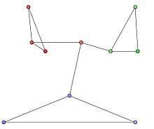
We consider an undirected network with 10 nodes and 12 edges and the following adjacency matrix.

Fig 1. Sample Network corresponding to the Adjacency matrix with 10 nodes, 12 edges.

Fig 2. Network partitions that maximize Q. Maximum Q=0.4896

The communities in the graph are represented by the red, green and blue node clusters in Fig 1. The optimal community partitions are depicted in Fig 2.

An alternative formulation of the modularity, useful particularly in spectral optimization algorithms, is as follows.[1] Define S_vr to be 1 if vertex v belongs to group r and zero otherwise. Then

${\displaystyle \delta (c_{v},c_{w})=\sum _{r}S_{vr}S_{wr}}$

and hence

${\displaystyle Q={\frac {1}{2m}}\sum _{vw}\sum _{r}\left[A_{vw}-{\frac {k_{v}k_{w}}{2m}}\right]S_{vr}S_{wr}={\frac {1}{2m}}\mathrm {Tr} (\mathbf {S} ^{\mathrm {T} }\mathbf {BS} ),}$

where S is the (non-square) matrix having elements S_vr and B is the so-called modularity matrix, which has elements

${\displaystyle B_{vw}=A_{vw}-{\frac {k_{v}k_{w}}{2m}}.}$

All rows and columns of the modularity matrix sum to zero, which means that the modularity of an undivided network is also always zero.

For networks divided into just two communities, one can alternatively define s_v = ±1 to indicate the community to which node v belongs, which then leads to

${\displaystyle Q={1 \over 4m}\sum _{vw}B_{vw}s_{v}s_{w}={1 \over 4m}\mathbf {s} ^{\mathrm {T} }\mathbf {Bs} ,}$

where s is the column vector with elements s_v.[1]

This function has the same form as the Hamiltonian of an Ising spin glass, a connection that has been exploited to create simple computer algorithms, for instance using simulated annealing, to maximize the modularity. The general form of the modularity for arbitrary numbers of communities is equivalent to a Potts spin glass and similar algorithms can be developed for this case also.[7]

Modularity compares the number of edges inside a cluster with the expected number of edges that one would find in the cluster if the network were a random network with the same number of nodes and where each node keeps its degree, but edges are otherwise randomly attached. This random null model implicitly assumes that each node can get attached to any other node of the network. This assumption is however unreasonable if the network is very large, as the horizon of a node includes a small part of the network, ignoring most of it. Moreover, this implies that the expected number of edges between two groups of nodes decreases if the size of the network increases. So, if a network is large enough, the expected number of edges between two groups of nodes in modularity's null model may be smaller than one. If this happens, a single edge between the two clusters would be interpreted by modularity as a sign of a strong correlation between the two clusters, and optimizing modularity would lead to the merging of the two clusters, independently of the clusters' features. So, even weakly interconnected complete graphs, which have the highest possible density of internal edges, and represent the best identifiable communities, would be merged by modularity optimization if the network were sufficiently large.[8] For this reason, optimizing modularity in large networks would fail to resolve small communities, even when they are well defined. This bias is inevitable for methods like modularity optimization, which rely on a global null model.[9]

There are two main approaches which try to solve the resolution limit within the modularity context: the addition of a resistance r to every node, in the form of a self-loop, which increases (r>0) or decreases (r<0) the aversion of nodes to form communities;[10] or the addition of a parameter γ>0 in front of the null-case term in the definition of modularity, which controls the relative importance between internal links of the communities and the null model.[7] Optimizing modularity for values of these parameters in their respective appropriate ranges, it is possible to recover the whole mesoscale of the network, from the macroscale in which all nodes belong to the same community, to the microscale in which every node forms its own community, hence the name multiresolution methods. However, it has been shown that these methods have limitations when communities are very heterogeneous in size.[11]

Percolation theory on modular networks have been studied by several authors[12] [13].

Spreading of epidemic has been studied recently on modular networks (networks with communities)[14]. Since a disease spreading in one country could become a pandemic with a potential worldwide humanitarian and economic impact, it is important to develop models to estimate the probability of a worldwide pandemic. A very recent example is the coronavirus that initiated in China (end of 2019) and spread globally. In this paper[14], a model is proposed for disease spreading in a structural modular complex network (having communities) and study how the number of bridge nodes n that connect communities affects disease spread and criterion to announce pandemic.

• Complex network
• Community structure
• Null model
• Percolation theory

References

- Newman, M. E. J. (2006). "Modularity and community structure in networks". Proceedings of the National Academy of Sciences of the United States of America. 103 (23): 8577–8696. arXiv:physics/0602124. Bibcode:2006PNAS..103.8577N. doi:10.1073/pnas.0601602103. PMC 1482622. PMID 16723398.
- Newman, M. E. J. (2007). Palgrave Macmillan, Basingstoke (eds.). "Mathematics of networks". The New Palgrave Encyclopedia of Economics (2 ed.).CS1 maint: uses editors parameter (link)
- Brandes, U.; Delling, D.; Gaertler, M.; Gorke, R.; Hoefer, M.; Nikoloski, Z.; Wagner, D. (February 2008). "On Modularity Clustering". IEEE Transactions on Knowledge and Data Engineering. 20 (2): 172–188. doi:10.1109/TKDE.2007.190689.
- van der Hofstad, Remco (2013). "Chapter 7" (PDF). Random Graphs and Complex Networks.
- "NetworkScience". Albert-László Barabási. Retrieved 2020-03-20.
- Clauset, Aaron and Newman, M. E. J. and Moore, Cristopher (2004). "Finding community structure in very large networks". Phys. Rev. E. 70 (6): 066111. arXiv:cond-mat/0408187. Bibcode:2004PhRvE..70f6111C. doi:10.1103/PhysRevE.70.066111. PMID 15697438.CS1 maint: multiple names: authors list (link)
- Joerg Reichardt & Stefan Bornholdt (2006). "Statistical mechanics of community detection". Physical Review E. 74 (1): 016110. arXiv:cond-mat/0603718. Bibcode:2006PhRvE..74a6110R. doi:10.1103/PhysRevE.74.016110. PMID 16907154.
- Santo Fortunato & Marc Barthelemy (2007). "Resolution limit in community detection". Proceedings of the National Academy of Sciences of the United States of America. 104 (1): 36–41. arXiv:physics/0607100. Bibcode:2007PNAS..104...36F. doi:10.1073/pnas.0605965104. PMC 1765466. PMID 17190818.
- J.M. Kumpula; J. Saramäki; K. Kaski & J. Kertész (2007). "Limited resolution in complex network community detection with Potts model approach". European Physical Journal B. 56 (1): 41–45. arXiv:cond-mat/0610370. Bibcode:2007EPJB...56...41K. doi:10.1140/epjb/e2007-00088-4.
- Alex Arenas, Alberto Fernández and Sergio Gómez (2008). "Analysis of the structure of complex networks at different resolution levels". New Journal of Physics. 10 (5): 053039. arXiv:physics/0703218. Bibcode:2008NJPh...10e3039A. doi:10.1088/1367-2630/10/5/053039.
- Andrea Lancichinetti & Santo Fortunato (2011). "Limits of modularity maximization in community detection". Physical Review E. 84 (6): 066122. arXiv:1107.1155. Bibcode:2011PhRvE..84f6122L. doi:10.1103/PhysRevE.84.066122. PMID 22304170.
- Shai, S; Kenett, D.Y; Kenett, Y.N; Faust, M; Dobson, S; Havlin, S. (2015). "Critical tipping point distinguishing two types of transitions in modular network structures". Phys. Rev. E. 92: 062805. doi:10.1103/PhysRevE.92.062805. PMID 26764742.
- Dong, Gaogao; Fan, Jingfang; Shekhtman, Louis M; Shai, Saray; Du, Ruijin; Tian, Lixin; Chen, Xiaosong; Stanley, H Eugene; Havlin, Shlomo (2018). "Resilience of networks with community structure behaves as if under an external field". Proceedings of the National Academy of Sciences. 115 (27): 6911–6915. arXiv:1805.01032. doi:10.1073/pnas.1801588115.
- Valdez, LD; Braunstein, LA; Havlin, S. "Epidemic spreading on modular networks: The fear to declare a pandemic". Phys. Rev. E. 101 (3): 032309. arXiv:1909.09695. doi:10.1103/PhysRevE.101.032309.