Graph (abstract data type)
In computer science, a graph is an abstract data type that is meant to implement the undirected graph and directed graph concepts from the field of graph theory within mathematics.
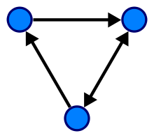
A graph data structure consists of a finite (and possibly mutable) set of vertices (also called nodes or points), together with a set of unordered pairs of these vertices for an undirected graph or a set of ordered pairs for a directed graph. These pairs are known as edges (also called links or lines), and for a directed graph are also known as arrows. The vertices may be part of the graph structure, or may be external entities represented by integer indices or references.
A graph data structure may also associate to each edge some edge value, such as a symbolic label or a numeric attribute (cost, capacity, length, etc.).
Operations
The basic operations provided by a graph data structure G usually include:[1]
adjacent(G, x, y): tests whether there is an edge from the vertex x to the vertex y;neighbors(G, x): lists all vertices y such that there is an edge from the vertex x to the vertex y;add_vertex(G, x): adds the vertex x, if it is not there;remove_vertex(G, x): removes the vertex x, if it is there;add_edge(G, x, y): adds the edge from the vertex x to the vertex y, if it is not there;remove_edge(G, x, y): removes the edge from the vertex x to the vertex y, if it is there;get_vertex_value(G, x): returns the value associated with the vertex x;set_vertex_value(G, x, v): sets the value associated with the vertex x to v.
Structures that associate values to the edges usually also provide:[1]
get_edge_value(G, x, y): returns the value associated with the edge (x, y);set_edge_value(G, x, y, v): sets the value associated with the edge (x, y) to v.
Representations
Different data structures for the representation of graphs are used in practice:
- Adjacency list[2]
- Vertices are stored as records or objects, and every vertex stores a list of adjacent vertices. This data structure allows the storage of additional data on the vertices. Additional data can be stored if edges are also stored as objects, in which case each vertex stores its incident edges and each edge stores its incident vertices.
- Adjacency matrix[3]
- A two-dimensional matrix, in which the rows represent source vertices and columns represent destination vertices. Data on edges and vertices must be stored externally. Only the cost for one edge can be stored between each pair of vertices.
- Incidence matrix[4]
- A two-dimensional Boolean matrix, in which the rows represent the vertices and columns represent the edges. The entries indicate whether the vertex at a row is incident to the edge at a column.
The following table gives the time complexity cost of performing various operations on graphs, for each of these representations, with |V | the number of vertices and |E | the number of edges. In the matrix representations, the entries encode the cost of following an edge. The cost of edges that are not present are assumed to be ∞.
| Adjacency list | Adjacency matrix | Incidence matrix | |
|---|---|---|---|
| Store graph | |||
| Add vertex | |||
| Add edge | |||
| Remove vertex | |||
| Remove edge | |||
| Are vertices x and y adjacent (assuming that their storage positions are known)? | |||
| Remarks | Slow to remove vertices and edges, because it needs to find all vertices or edges | Slow to add or remove vertices, because matrix must be resized/copied | Slow to add or remove vertices and edges, because matrix must be resized/copied |


Adjacency lists are generally preferred because they efficiently represent sparse graphs. An adjacency matrix is preferred if the graph is dense, that is the number of edges |E | is close to the number of vertices squared, |V |2, or if one must be able to quickly look up if there is an edge connecting two vertices.[5][6]
Parallel Graph Representations
The parallelization of graph problems faces significant challenges: Data-driven computations, unstructured problems, poor locality and high data access to computation ratio.[7][8] The graph representation used for parallel architectures plays a significant role in facing those challenges. Poorly chosen representations may unnecessarily drive up the communication cost of the algorithm, which will decrease its scalability. In the following, shared and distributed memory architectures are considered.
Shared memory
In the case of a shared memory model, the graph representations used for parallel processing are the same as in the sequential case,[9] since parallel read-only access to the graph representation (e.g. an adjacency list) is efficient in shared memory.
Distributed Memory
In the distributed memory model, the usual approach is to partition the vertex set of the graph into sets . Here, is the amount of available processing elements (PE). The vertex set partitions are then distributed to the PEs with matching index, additionally to the corresponding edges. Every PE has its own subgraph representation, where edges with an endpoint in another partition require special attention. For standard communication interfaces like MPI, the ID of the PE owning the other endpoint has to be identifiable. During computation in a distributed graph algorithms, passing information along these edges implies communication.[9]


Partitioning the graph needs to be done carefully - there is a trade-off between low communication and even size partitioning[10] But partitioning a graph is a NP-hard problem, so it is not feasible to calculate them. Instead, the following heuristics are used.
1D partitioning: Every processor gets vertices and the corresponding outgoing edges. This can be understood as a row-wise or column-wise decomposition of the adjacency matrix. For algorithms operating on this representation, this requires an All-to-All communication step as well as message buffer sizes, as each PE potentially has outgoing edges to every other PE.[11]


2D partitioning: Every processor gets a submatrix of the adjacency matrix. Assume the processors are aligned in a rectangle , where and are the amount of processing elements in each row and column, respectively. Then each processor gets a submatrix of the adjacency matrix of dimension . This can be visualized as a checkerboard pattern in a matrix.[11] Therefore, each processing unit can only have outgoing edges to PEs in the same row and column. This bounds the amount of communication partners for each PE to out of possible ones.


See also
- Graph traversal for graph walking strategies
- Graph database for graph (data structure) persistency
- Graph rewriting for rule based transformations of graphs (graph data structures)
- Graph drawing software for software, systems, and providers of systems for drawing graphs
References
- See, e.g. Goodrich & Tamassia (2015), Section 13.1.2: Operations on graphs, p. 360. For a more detailed set of operations, see Mehlhorn, K.; Näher, S. (1999), "Chapter 6: Graphs and their data structures", LEDA: A platform for combinatorial and geometric computing, Cambridge University Press, pp. 240–282.
- Cormen et al. (2001), pp. 528–529; Goodrich & Tamassia (2015), pp. 361-362.
- Cormen et al. (2001), pp. 529–530; Goodrich & Tamassia (2015), p. 363.
- Cormen et al. (2001), Exercise 22.1-7, p. 531.
- Cormen, Thomas H.; Leiserson, Charles E.; Rivest, Ronald L.; Stein, Clifford (2001), "Section 22.1: Representations of graphs", Introduction to Algorithms (Second ed.), MIT Press and McGraw-Hill, pp. 527–531, ISBN 0-262-03293-7.
- Goodrich, Michael T.; Tamassia, Roberto (2015), "Section 13.1: Graph terminology and representations", Algorithm Design and Applications, Wiley, pp. 355–364.
- Bader, David; Meyerhenke, Henning; Sanders, Peter; Wagner, Dorothea (January 2013). Graph Partitioning and Graph Clustering. Contemporary Mathematics. 588. American Mathematical Society. doi:10.1090/conm/588/11709. ISBN 978-0-8218-9038-7.
- LUMSDAINE, ANDREW; GREGOR, DOUGLAS; HENDRICKSON, BRUCE; BERRY, JONATHAN (March 2007). "CHALLENGES IN PARALLEL GRAPH PROCESSING". Parallel Processing Letters. 17 (01): 5–20. doi:10.1142/s0129626407002843. ISSN 0129-6264.
- Sanders, Peter; Mehlhorn, Kurt; Dietzfelbinger, Martin; Dementiev, Roman (2019). Sequential and Parallel Algorithms and Data Structures: The Basic Toolbox. Springer International Publishing. ISBN 978-3-030-25208-3.
- "Parallel Processing of Graphs" (PDF).
- "Parallel breadth-first search on distributed memory systems | Proceedings of 2011 International Conference for High Performance Computing, Networking, Storage and Analysis". dl.acm.org. doi:10.1145/2063384.2063471. Retrieved 2020-02-06.
External links
| Wikimedia Commons has media related to Graph (abstract data type). |
- Boost Graph Library: a powerful C++ graph library s.a. Boost (C++ libraries)
- Networkx: a Python graph library
- GraphMatcher a java program to align directed/undirected graphs.
- GraphBLAS A specification for a library interface for operations on graphs, with a particular focus on sparse graphs.