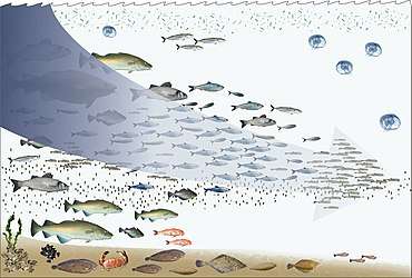
Marine food web
Compared to terrestrial environments, marine environments have biomass pyramids which are inverted at the base. In particular, the biomass of consumers (copepods, krill, shrimp, forage fish) is larger than the biomass of primary producers. This happens because the ocean's primary producers are tiny phytoplankton which grow and reproduce rapidly, so a small mass can have a fast rate of primary production. In contrast, terrestrial primary producers, such as mature forests, grow and reproduce slowly, so a much larger mass is needed to achieve the same rate of primary production.
| Part of a series of overviews on |
| Marine life |
|---|
|
|
Because of this inversion, it is the zooplankton that make up most of the marine animal biomass. As primary consumers, zooplankton are the crucial link between the primary producers (mainly phytoplankton) and the rest of the marine food web (secondary consumers).[1]
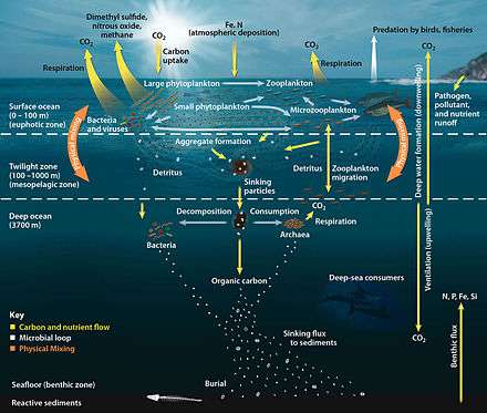
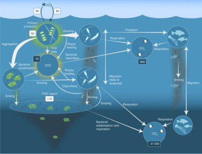
If phytoplankton dies before it is eaten, it descends through the euphotic zone as part of the marine snow and settles into the depths of sea. In this way, phytoplankton sequester about 2 billion tons of carbon dioxide into the ocean each year, causing the ocean to become a sink of carbon dioxide holding about 90% of all sequestered carbon.[2] The ocean produces about half of the world's oxygen and stores 50 times more carbon dioxide than the atmosphere.[3]
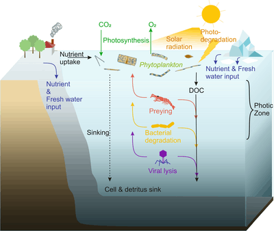
An ecosystem cannot be understood without knowledge of how its food web determines the flow of materials and energy. Phytoplankton autotrophically produces biomass by converting inorganic compounds into organic ones. In this way, phytoplankton functions as the foundation of the marine food web by supporting all other life in the ocean. The second central process in the marine food web is the microbial loop. This loop degrades marine bacteria and archaea, remineralises organic and inorganic matter, and then recycles the products either within the pelagic food web or by depositing them as sediment on the seafloor.[4]
Food chains and trophic levels
| marine food chain (typical) |
|---|
|
|
| ↓ |
| phytoplankton |
| ↓ |
| herbivorous zooplankton |
| ↓ |
| carnivorous zooplankton |
| ↓ |
|
|
| ↓ |
|
|
Food webs are built from food chains. All forms of life in the sea have the potential to become food for another life form. In the ocean, a food chain typically starts with energy from the sun powering phytoplankton, and follows a course such as:
phytoplankton → herbivorous zooplankton → carnivorous zooplankton → filter feeder → predatory vertebrate
Phytoplankton don't need other organisms for food, because they have the ability to manufacture their own food directly from inorganic carbon, using sunlight as their energy source. This process is called photosynthesis, and results in the phytoplankton converting naturally occurring carbon into protoplasm. For this reason, phytoplankton are said to be the primary producers at the bottom or the first level of the marine food chain. Since they are at the first level they are said to have a trophic level of 1 (from the Greek trophē meaning food). Phytoplankton are then consumed at the next trophic level in the food chain by microscopic animals called zooplankton.
Zooplankton comprise the second trophic level in the food chain, and include microscopic one-celled organisms called protozoa as well as small crustaceans, such as copepods and krill, and the larva of fish, squid, lobsters and crabs. Organisms at this level can be thought of as primary consumers.
In turn, the smaller herbivorous zooplankton are consumed by larger carnivorous zooplankters, such as larger predatory protozoa and krill, and by forage fish, which are small, schooling, filter-feeding fish. This makes up the third trophic level in the food chain.

The fourth trophic level consists of predatory fish, marine mammals and seabirds that consume forage fish. Examples are swordfish, seals and gannets.
Apex predators, such as orcas, which can consume seals, and shortfin mako sharks, which can consume swordfish, make up a fifth trophic level. Baleen whales can consume zooplankton and krill directly, leading to a food chain with only three or four trophic levels.
In practice, trophic levels are not usually simple integers because the same consumer species often feeds across more than one trophic level.[8][9] For example a large marine vertebrate may eat smaller predatory fish but may also eat filter feeders; the stingray eats crustaceans, but the hammerhead eats both crustaceans and stingrays. Animals can also eat each other; the cod eats smaller cod as well as crayfish, and crayfish eat cod larvae. The feeding habits of a juvenile animal, and, as a consequence, its trophic level, can change as it grows up.
The fisheries scientist Daniel Pauly sets the values of trophic levels to one in primary producers and detritus, two in herbivores and detritivores (primary consumers), three in secondary consumers, and so on. The definition of the trophic level, TL, for any consumer species is:[10]

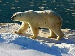
where is the fractional trophic level of the prey j, and represents the fraction of j in the diet of i. In the case of marine ecosystems, the trophic level of most fish and other marine consumers takes value between 2.0 and 5.0. The upper value, 5.0, is unusual, even for large fish,[11] though it occurs in apex predators of marine mammals, such as polar bears and killer whales.[12] As a point of contrast, humans have a mean trophic level of about 2.21, about the same as a pig or an anchovy.[13][14]


Primary producers
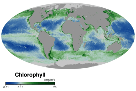
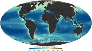
At the base of the ocean food web are single-celled algae and other plant-like organisms known as phytoplankton. Like plants on land, phytoplankton use chlorophyll and other light-harvesting pigments to carry out photosynthesis, absorbing atmospheric carbon dioxide to produce sugars for fuel. Chlorophyll in the water changes the way it reflects and absorbs sunlight, allowing scientists to map the amount and location of phytoplankton. These measurements give scientists valuable insights into the health of the ocean environment, and help scientists study the ocean carbon cycle.[15]
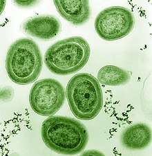
Among the phytoplankton are members from a phylum of bacteria called cyanobacteria. Marine cyanobacteria include the smallest known photosynthetic organisms. The smallest of all, Prochlorococcus, is just 0.5 to 0.8 micrometres across.[16] In terms of individual numbers, Prochlorococcus is possibly the most plentiful species on Earth: a single millilitre of surface seawater can contain 100,000 cells or more. Worldwide there are estimated to be several octillion (1027) individuals.[17] Prochlorococcus is ubiquitous between 40°N and 40°S and dominates in the oligotrophic (nutrient poor) regions of the oceans.[18] The bacterium accounts for about 20% of the oxygen in the Earth's atmosphere.[19]
- Phytoplankton form the base of the ocean foodchain
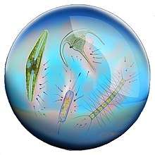
 Phytoplankton
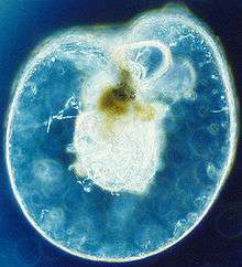 Dinoflagellate
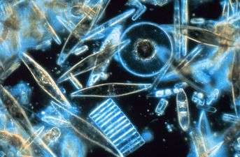 Diatoms
In oceans, most primary production is performed by algae. This is a contrast to on land, where most primary production is performed by vascular plants. Algae ranges from single floating cells to attached seaweeds, while vascular plants are represented in the ocean by groups such as the seagrasses. Larger producers, such as seagrasses and seaweeds, are mostly confined to the littoral zone and shallow waters, where they attach to the underlying substrate and are still within the photic zone. But most of the primary production by algae is performed by the phytoplankton.
Thus, in ocean environments, the first bottom trophic level is occupied principally by phytoplankton, microscopic drifting organisms, mostly one-celled algae, that float in the sea. Most phytoplankton are too small to be seen individually with the unaided eye. They can appear as a green discoloration of the water when they are present in high enough numbers. Since they increase their biomass mostly through photosynthesis they live in the sun-lit surface layer (euphotic zone) of the sea.
The most important groups of phytoplankton include the diatoms and dinoflagellates. Diatoms are especially important in oceans, where according to some estimates they contribute up to 45% of the total ocean's primary production.[20] Diatoms are usually microscopic, although some species can reach up to 2 millimetres in length.
Primary consumers
The second trophic level (primary consumers) is occupied by zooplankton which feed off the phytoplankton. Together with the phytoplankton, they form the base of the food pyramid that supports most of the world's great fishing grounds. Zooplankton are tiny animals found with the phytoplankton in oceanic surface waters, and include tiny crustaceans, and fish larvae and fry (recently hatched fish). Most zooplankton are filter feeders, and they use appendages to strain the phytoplankton in the water. Some larger zooplankton also feed on smaller zooplankton. Some zooplankton can jump about a bit to avoid predators, but they can't really swim. Like phytoplankton, they float with the currents, tides and winds instead. Zooplanktons can reproduce rapidly, their populations can increase up to thirty percent a day under favourable conditions. Many live short and productive lives and reach maturity quickly.
- Zooplankton form a second level in the ocean food chain
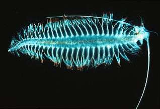 Segmented worm
 Tiny shrimp-like crustaceans
 Juvenile planktonic squid
Particularly important groups of zooplankton are the copepods and krill. Copepods are a group of small crustaceans found in ocean and freshwater habitats. They are the biggest source of protein in the sea,[21] and are important prey for forage fish. Krill constitute the next biggest source of protein. Krill are particularly large predator zooplankton which feed on smaller zooplankton. This means they really belong to the third trophic level, secondary consumers, along with the forage fish.

Together, phytoplankton and zooplankton make up most of the plankton in the sea. Plankton is the term applied to any small drifting organisms that float in the sea (Greek planktos = wanderer or drifter). By definition, organisms classified as plankton are unable to swim against ocean currents; they cannot resist the ambient current and control their position. In ocean environments, the first two trophic levels are occupied mainly by plankton. Plankton are divided into producers and consumers. The producers are the phytoplankton (Greek phyton = plant) and the consumers, who eat the phytoplankton, are the zooplankton (Greek zoon = animal).
Jellyfish are slow swimmers, and most species form part of the plankton. Traditionally jellyfish have been viewed as trophic dead ends, minor players in the marine food web, gelatinous organisms with a body plan largely based on water that offers little nutritional value or interest for other organisms apart from a few specialised predators such as the ocean sunfish and the leatherback sea turtle.[23][22] That view has recently been challenged. Jellyfish, and more generally gelatinous zooplankton which include salps and ctenophores, are very diverse, fragile with no hard parts, difficult to see and monitor, subject to rapid population swings and often live inconveniently far from shore or deep in the ocean. It is difficult for scientists to detect and analyse jellyfish in the guts of predators, since they turn to mush when eaten and are rapidly digested.[23] But jellyfish bloom in vast numbers, and it has been shown they form major components in the diets of tuna, spearfish and swordfish as well as various birds and invertebrates such as octopus, sea cucumbers, crabs and amphipods.[24][22] "Despite their low energy density, the contribution of jellyfish to the energy budgets of predators may be much greater than assumed because of rapid digestion, low capture costs, availability, and selective feeding on the more energy-rich components. Feeding on jellyfish may make marine predators susceptible to ingestion of plastics."[22]
Higher order consumers

- Marine invertebrates
- Fish
- Forage fish: Forage fish occupy central positions in the ocean food webs. The organisms it eats are at a lower trophic level, and the organisms that eat it are at a higher trophic level. Forage fish occupy middle levels in the food web, serving as a dominant prey to higher level fish, seabirds and mammals.[25]
- Predator fish
- Ground fish
- Other marine vertebrates
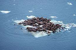
In 2010 researchers found whales carry nutrients from the depths of the ocean back to the surface using a process they called the whale pump.[26] Whales feed at deeper levels in the ocean where krill is found, but return regularly to the surface to breathe. There whales defecate a liquid rich in nitrogen and iron. Instead of sinking, the liquid stays at the surface where phytoplankton consume it. In the Gulf of Maine the whale pump provides more nitrogen than the rivers.[27]
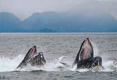 Humpback whales lunge from below to feed on forage fish
%2C_Belmont_-_geograph.org.uk_-_529175.jpg) Gannets plunge dive from above to catch forage fish
Gannets plunge dive from above to catch forage fish
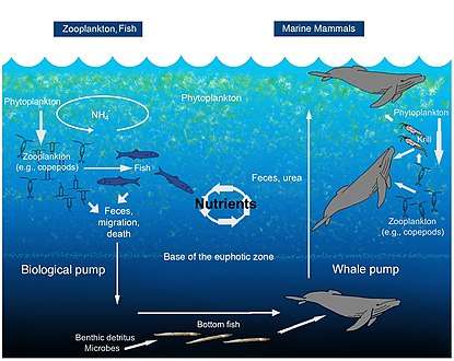 Whale pump nutrient cycle
Microorganisms
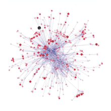
There has been increasing recognition in recent years that marine microorganisms play much bigger roles in marine ecosystems than was previously thought. Developments in metagenomics gives researchers an ability to reveal previously hidden diversities of microscopic life, offering a powerful lens for viewing the microbial world and the potential to revolutionise understanding of the living world.[29] Metabarcoding dietary analysis techniques are being used to reconstruct food webs at higher levels of taxonomic resolution and are revealing deeper complexities in the web of interactions.[30]
Microorganisms play key roles in marine food webs. The viral shunt pathway is a mechanism that prevents marine microbial particulate organic matter (POM) from migrating up trophic levels by recycling them into dissolved organic matter (DOM), which can be readily taken up by microorganisms.[31] Viral shunting helps maintain diversity within the microbial ecosystem by preventing a single species of marine microbe from dominating the micro-environment.[32] The DOM recycled by the viral shunt pathway is comparable to the amount generated by the other main sources of marine DOM.[33]
as imaged by a satellite in 2011

.jpg)

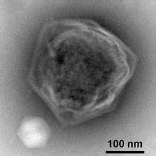
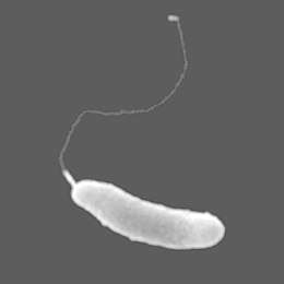
A giant marine virus CroV infects and causes the death by lysis of the marine zooflagellate Cafeteria roenbergensis.[37] This impacts coastal ecology because Cafeteria roenbergensis feeds on bacteria found in the water. When there are low numbers of Cafeteria roenbergensis due to extensive CroV infections, the bacterial populations rise exponentially.[38] The impact of CroV on natural populations of C. roenbergensis remains unknown; however, the virus has been found to be very host specific, and does not infect other closely related organisms.[39] Cafeteria roenbergensis is also infected by a second virus, the Mavirus virophage, which is a satellite virus, meaning it is able to replicate only in the presence of another specific virus, in this case in the presence of CroV.[40] This virus interferes with the replication of CroV, which leads to the survival of C. roenbergensis cells. Mavirus is able to integrate into the genome of cells of C. roenbergensis, and thereby confer immunity to the population.[41]
Fungi
- Amend, A., Burgaud, G., Cunliffe, M., Edgcomb, V.P., Ettinger, C.L., Gutiérrez, M.H., Heitman, J., Hom, E.F., Ianiri, G., Jones, A.C. and Kagami, M. (2019) "Fungi in the marine environment: Open questions and unsolved problems". MBio, 10(2): e01189-18. doi:10.1128/mBio.01189-18.

By habitat
Coastal webs

- Byrnes, J.E., Reynolds, P.L. and Stachowicz, J.J. (2007) "Invasions and extinctions reshape coastal marine food webs". PloS one, 2(3): e295. doi:10.1371/journal.pone.0000295

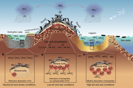
The key nutrients determining eutrophication are nitrogen in coastal waters and phosphorus in lakes. Both are found in high concentrations in guano (seabird feces), which acts as a fertilizer for the surrounding ocean or an adjacent lake. Uric acid is the dominant nitrogen compound, and during its mineralization different nitrogen forms are produced. In the diagram on the right: (1) ammonification produces NH3 and NH4+, and (2) nitrification produces NO3− by NH4+ oxidation. Under the alkaline conditions, typical of the seabird feces, the NH3 is rapidly volatised (3) and transformed to NH4+, which is transported out of the colony, and through wet-deposition exported to distant ecosystems, which are eutrophised (4). The phosphorus cycle is simpler and has reduced mobility. This element is found in a number of chemical forms in the seabird fecal material, but the most mobile and bioavailable is orthophosphate, which can be leached by subterranean or superficial waters (5).[47]
DNA barcoding can be used to construct food web structures with better taxonomic resolution at the web nodes. This provides more specific species identification and greater clarity about exactly who eats whom. "DNA barcodes and DNA information may allow new approaches to the construction of larger interaction webs, and overcome some hurdles to achieving adequate sample size".[30]
A newly applied method for species identification is DNA metabarcoding. Species identification via morphology is relatively difficult and requires a lot of time and expertise.[54][55] High throughput sequencing DNA metabarcoding enables taxonomic assignment and therefore identification for the complete sample regarding the group specific primers chosen for the previous DNA amplification.
At the ocean surface

Ocean surface habitats sit at the interface between the atmosphere and the ocean. The biofilm-like habitat at the surface of the ocean harbours surface-dwelling microorganisms, commonly referred to as neuston. This vast air–water interface sits at the intersection of major air–water exchange processes spanning more than 70% of the global surface area . Bacteria in the surface microlayer of the ocean, called bacterioneuston, are of interest due to practical applications such as air-sea gas exchange of greenhouse gases, production of climate-active marine aerosols, and remote sensing of the ocean.[56] Of specific interest is the production and degradation of surfactants (surface active materials) via microbial biochemical processes. Major sources of surfactants in the open ocean include phytoplankton,[57] terrestrial runoff, and deposition from the atmosphere.[56]
Unlike coloured algal blooms, surfactant-associated bacteria may not be visible in ocean colour imagery. Having the ability to detect these "invisible" surfactant-associated bacteria using synthetic aperture radar has immense benefits in all-weather conditions, regardless of cloud, fog, or daylight.[56] This is particularly important in very high winds, because these are the conditions when the most intense air-sea gas exchanges and marine aerosol production take place. Therefore, in addition to colour satellite imagery, SAR satellite imagery may provide additional insights into a global picture of biophysical processes at the boundary between the ocean and atmosphere, air-sea greenhouse gas exchanges and production of climate-active marine aerosols.[56]
Deep ocean webs
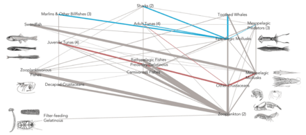
- The mesopelagic web
- Mesopelagic food web
 Impact of mesopelagic species on the global carbon budget [58]
DVM = diel vertical migration NM = non-migration
Scientists are starting to explore in more detail the largely unknown twilight zone of the mesopelagic, 200 to 1,000 metres deep. This layer is responsible for removing about 4 billion tonnes of carbon dioxide from the atmosphere each year. The mesopelagic layer is inhabited by most of the marine fish biomass.[59]
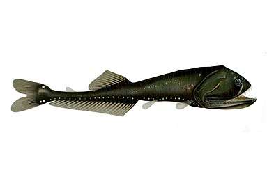 Mesopelagic bristlemouths may be the most abundant vertebrates on the planet, though little is known about them.[59]
 Gelatinous predators like this narcomedusan consume the greatest diversity of mesopelagic prey
- Fish in the twilight cast new light on ocean ecosystem The Conversation, 10 February 2014.
- An Ocean Mystery in the Trillions The New York Times, 29 June 2015.
- Mesopelagic fishes - Malaspina circumnavigation expedition of 2010.[60][61]
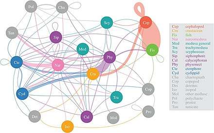
According to a 2017 study, narcomedusae consume the greatest diversity of mesopelagic prey, followed by physonect siphonophores, ctenophores and cephalopods. The importance of the so called "jelly web" is only beginning to be understood, but it seems medusae, ctenophores and siphonophores can be key predators in deep pelagic food webs with ecological impacts similar to predator fish and squid. Traditionally gelatinous predators were thought ineffectual providers of marine trophic pathways, but they appear to have substantial and integral roles in deep pelagic food webs.[62] Diel vertical migration, an important active transport mechanism, allows mesozooplankton to sequester carbon dioxide from the atmosphere as well as supply carbon needs for other mesopelagic organisms.[63]
- The deep pelagic web
- Seeps and vents


A 2020 study reported that by 2050 global warming could be spreading in the deep ocean seven times faster than it is now, even if emissions of greenhouse gases are cut. Warming in mesopelagic and deeper layers could have major consequences for the deep ocean food web, since ocean species will need to move to stay at survival temperatures.[69][70]
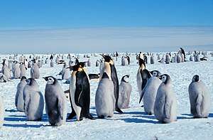
Polar webs
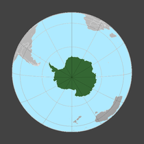
surrounded by oceans
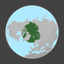
surrounded by landmasses
Arctic and Antarctic marine systems have very different topographical structures and as a consequence have very different food web structures.[71] Both Arctic and Antarctic pelagic food webs have characteristic energy flows controlled largely by a few key species. But there is no single generic web for either. Alternative pathways are important for resilience and maintaining energy flows. However, these more complicated alternatives provide less energy flow to upper trophic-level species. "Food-web structure may be similar in different regions, but the individual species that dominate mid-trophic levels vary across polar regions".[72]

- Arctic


The Arctic food web is complex. The loss of sea ice can ultimately affect the entire food web, from algae and plankton to fish to mammals. The impact of climate change on a particular species can ripple through a food web and affect a wide range of other organisms... Not only is the decline of sea ice impairing polar bear populations by reducing the extent of their primary habitat, it is also negatively impacting them via food web effects. Declines in the duration and extent of sea ice in the Arctic leads to declines in the abundance of ice algae, which thrive in nutrient-rich pockets in the ice. These algae are eaten by zooplankton, which are in turn eaten by Arctic cod, an important food source for many marine mammals, including seals. Seals are eaten by polar bears. Hence, declines in ice algae can contribute to declines in polar bear populations.[73]

Gray arrows: flow of carbon to heterotrophs
Green arrows: major pathways of carbon flow to or from mixotrophs
HCIL: heterotrophic ciliates; MCIL: mixotrophic ciliates; HNF: heterotrophic nanoflagellates; DOC: dissolved organic carbon; HDIN: heterotrophic dinoflagellates [74]
- Antarctic
.jpg) Antarctic jellyfish Diplulmaris antarctica under the ice
Antarctic jellyfish Diplulmaris antarctica under the ice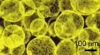 Colonies of the alga Phaeocystis antarctica, an important phytoplankter of the Ross Sea that dominates early season blooms after the sea ice retreats and exports significant carbon.[75]
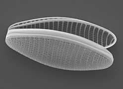 The pennate diatom Fragilariopsis kerguelensis, found throughout the Antarctic Circumpolar Current, is a key driver of the global silicate pump.[76]
and carbon masses (Gt C) in dark boxes


Foundation and keystone species
.jpg)
.jpg)
Foundation species are species that have a dominant role structuring an ecological community, shaping its environment and defining its ecosystem. Such ecosystems are often named after the foundation species, such as seagrass meadows, oyster beds, coral reefs, kelp forests and mangrove forests.[83] For example, the red mangrove is a common foundation species in mangrove forests. The mangrove’s root provides nursery grounds for young fish, such as snapper.[84] A foundation species can occupy any trophic level in a food web but tend to be a producer. [85]
The term was coined in 1972 by Paul K. Dayton,[86] who applied it to certain members of marine invertebrate and algae communities. It was clear from studies in several locations that there were a small handful of species whose activities had a disproportionate effect on the rest of the marine community and they were therefore key to the resilience of the community. Dayton’s view was that focusing on foundation species would allow for a simplified approach to more rapidly understand how a community as a whole would react to disturbances, such as pollution, instead of attempting the extremely difficult task of tracking the responses of all community members simultaneously.

Keystone species are species that have large effects, disproportionate to their numbers, within ecosystem food webs.[87] An ecosystem may experience a dramatic shift if a keystone species is removed, even though that species was a small part of the ecosystem by measures of biomass or productivity.[88]
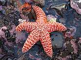
The concept of the keystone species was introduced in 1969 by the zoologist Robert T. Paine.[89][90] Paine developed the concept to explain his observations and experiments on the relationships between marine invertebrates of the intertidal zone (between the high and low tide lines), including starfish and mussels. Some sea stars prey on sea urchins, mussels, and other shellfish that have no other natural predators. If the sea star is removed from the ecosystem, the mussel population explodes uncontrollably, driving out most other species.[91]
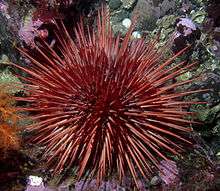
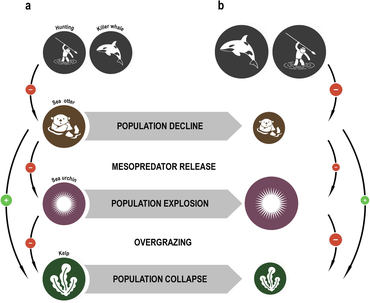
Sea otters limit the damage sea urchins inflict on kelp forests. When the sea otters of the North American west coast were hunted commercially for their fur, their numbers fell to such low levels that they were unable to control the sea urchin population. The urchins in turn grazed the holdfasts of kelp so heavily that the kelp forests largely disappeared, along with all the species that depended on them. Reintroducing the sea otters has enabled the kelp ecosystem to be restored.[92][93]
Cryptic interactions

Cryptic interactions, interactions which are "hidden in plain sight", occur throughout the marine planktonic foodweb but are currently largely overlooked by established methods, which mean large‐scale data collection for these interactions is limited. Despite this, current evidence suggests some of these interactions may have perceptible impacts on foodweb dynamics and model results. Incorporation of cryptic interactions into models is especially important for those interactions involving the transport of nutrients or energy.[94]
Simplifications such as “zooplankton consume phytoplankton,” “phytoplankton take up inorganic nutrients,” “gross primary production determines the amount of carbon available to the foodweb,” etc. have helped scientists explain and model general interactions in the aquatic environment. Traditional methods have focused on quantifying and qualifying these generalizations, but rapid advancements in genomics, sensor detection limits, experimental methods, and other technologies in recent years have shown that generalization of interactions within the plankton community may be too simple. These enhancements in technology have exposed a number of interactions which appear as cryptic because bulk sampling efforts and experimental methods are biased against them.[94]
Complexity and stability
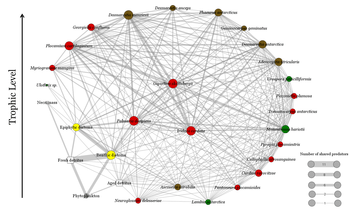
Food webs provide a framework within which a complex network of predator–prey interactions can be organised. A food web model is a network of food chains. Each food chain starts with a primary producer or autotroph, an organism, such as an alga or a plant, which is able to manufacture its own food. Next in the chain is an organism that feeds on the primary producer, and the chain continues in this way as a string of successive predators. The organisms in each chain are grouped into trophic levels, based on how many links they are removed from the primary producers. The length of the chain, or trophic level, is a measure of the number of species encountered as energy or nutrients move from plants to top predators.[97] Food energy flows from one organism to the next and to the next and so on, with some energy being lost at each level. At a given trophic level there may be one species or a group of species with the same predators and prey.[98]
In 1927, Charles Elton published an influential synthesis on the use of food webs, which resulted in them becoming a central concept in ecology.[99] In 1966, interest in food webs increased after Robert Paine's experimental and descriptive study of intertidal shores, suggesting that food web complexity was key to maintaining species diversity and ecological stability.[100] Many theoretical ecologists, including Robert May and Stuart Pimm, were prompted by this discovery and others to examine the mathematical properties of food webs. According to their analyses, complex food webs should be less stable than simple food webs.[101]:75–77[102]:64 The apparent paradox between the complexity of food webs observed in nature and the mathematical fragility of food web models is currently an area of intensive study and debate. The paradox may be due partially to conceptual differences between persistence of a food web and equilibrial stability of a food web.[101][102]
A trophic cascade can occur in a food web if a trophic level in the web is suppressed.
For example, a top-down cascade can occur if predators are effective enough in predation to reduce the abundance, or alter the behavior, of their prey, thereby releasing the next lower trophic level from predation. A top-down cascade is a trophic cascade where the top consumer/predator controls the primary consumer population. In turn, the primary producer population thrives. The removal of the top predator can alter the food web dynamics. In this case, the primary consumers would overpopulate and exploit the primary producers. Eventually there would not be enough primary producers to sustain the consumer population. Top-down food web stability depends on competition and predation in the higher trophic levels. Invasive species can also alter this cascade by removing or becoming a top predator. This interaction may not always be negative. Studies have shown that certain invasive species have begun to shift cascades; and as a consequence, ecosystem degradation has been repaired.[103][104] An example of a cascade in a complex, open-ocean ecosystem occurred in the northwest Atlantic during the 1980s and 1990s. The removal of Atlantic cod (Gadus morhua) and other ground fishes by sustained overfishing resulted in increases in the abundance of the prey species for these ground fishes, particularly smaller forage fishes and invertebrates such as the northern snow crab (Chionoecetes opilio) and northern shrimp (Pandalus borealis). The increased abundance of these prey species altered the community of zooplankton that serve as food for smaller fishes and invertebrates as an indirect effect.[105] Top-down cascades can be important for understanding the knock-on effects of removing top predators from food webs, as humans have done in many places through hunting and fishing.
In a bottom-up cascade, the population of primary producers will always control the increase/decrease of the energy in the higher trophic levels. Primary producers are plants, phytoplankton and zooplankton that require photosynthesis. Although light is important, primary producer populations are altered by the amount of nutrients in the system. This food web relies on the availability and limitation of resources. All populations will experience growth if there is initially a large amount of nutrients.[106][107]
Terrestrial comparisons
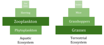
Compared to terrestrial biomass pyramids, aquatic pyramids are generally inverted at the base
.jpg)
.jpg)
Marine environments can have inversions in their biomass pyramids. In particular, the biomass of consumers (copepods, krill, shrimp, forage fish) is generally larger than the biomass of primary producers. This happens because the ocean's primary producers are mostly tiny phytoplankton which have r-strategist traits of growing and reproducing rapidly, so a small mass can have a fast rate of primary production. In contrast, many terrestrial primary producers, such as mature forests, have K-strategist traits of growing and reproducing slowly, so a much larger mass is needed to achieve the same rate of primary production.
Examples: The bristlecone pine can live for thousands of years, and has a very low production/biomass ratio. The cyanobacterium Prochlorococcus lives for about 24 hours, and has a very high production/biomass ratio.
.jpeg)

In oceans, most primary production is performed by algae. This is a contrast to on land, where most primary production is performed by vascular plants.
Aquatic producers, such as planktonic algae or aquatic plants, lack the large accumulation of secondary growth that exists in the woody trees of terrestrial ecosystems. However, they are able to reproduce quickly enough to support a larger biomass of grazers. This inverts the pyramid. Primary consumers have longer lifespans and slower growth rates that accumulates more biomass than the producers they consume. Phytoplankton live just a few days, whereas the zooplankton eating the phytoplankton live for several weeks and the fish eating the zooplankton live for several consecutive years.[110] Aquatic predators also tend to have a lower death rate than the smaller consumers, which contributes to the inverted pyramidal pattern. Population structure, migration rates, and environmental refuge for prey are other possible causes for pyramids with biomass inverted. Energy pyramids, however, will always have an upright pyramid shape if all sources of food energy are included, since this is dictated by the second law of thermodynamics."[111][112]
Comparison of productivity in marine and terrestrial ecosystems [113] | |||
|---|---|---|---|
| Ecosystem | Net primary productivity billion tonnes per year |
Total plant biomass billion tonnes |
Turnover time years |
Marine |
45–55 |
1–2 |
0.02–0.06 |
Terrestrial |
55–70 |
600–1000 |
9–20 |
Anthropogenic effects
- Overfishing
- Acidification
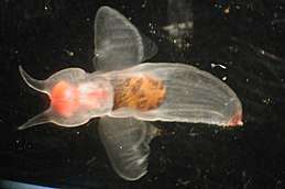
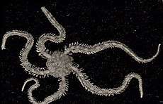
Pteropods and brittle stars together form the base of the Arctic food webs and both are seriously damaged by acidification. Pteropods shells dissolve with increasing acidification and brittle stars lose muscle mass when re-growing appendages.[115] Additionally the brittle star's eggs die within a few days when exposed to expected conditions resulting from Arctic acidification.[116] Acidification threatens to destroy Arctic food webs from the base up. Arctic waters are changing rapidly and are advanced in the process of becoming undersaturated with aragonite.[117] Arctic food webs are considered simple, meaning there are few steps in the food chain from small organisms to larger predators. For example, pteropods are "a key prey item of a number of higher predators – larger plankton, fish, seabirds, whales".[118]
.jpg)
- Climate change
"Our results show how future climate change can potentially weaken marine food webs through reduced energy flow to higher trophic levels and a shift towards a more detritus-based system, leading to food web simplification and altered producer–consumer dynamics, both of which have important implications for the structuring of benthic communities."[119][120]
"...increased temperatures reduce the vital flow of energy from the primary food producers at the bottom (e.g. algae), to intermediate consumers (herbivores), to predators at the top of marine food webs. Such disturbances in energy transfer can potentially lead to a decrease in food availability for top predators, which in turn, can lead to negative impacts for many marine species within these food webs... "Whilst climate change increased the productivity of plants, this was mainly due to an expansion of cyanobacteria (small blue-green algae)," said Mr Ullah. "This increased primary productivity does not support food webs, however, because these cyanobacteria are largely unpalatable and they are not consumed by herbivores. Understanding how ecosystems function under the effects of global warming is a challenge in ecological research. Most research on ocean warming involves simplified, short-term experiments based on only one or a few species."[120]


References
- U S Department of Energy (2008) Carbon Cycling and Biosequestration page 81, Workshop report DOE/SC-108, U.S. Department of Energy Office of Science.
- Campbell, Mike (22 June 2011). "The role of marine plankton in sequestration of carbon". EarthTimes. Retrieved 22 August 2014.
- Why should we care about the ocean? NOAA: National Ocean Service. Updated: 7 January 2020. Retrieved 1 March 2020.
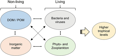
- Heinrichs, M.E., Mori, C. and Dlugosch, L. (2020) "Complex Interactions Between Aquatic Organisms and Their Chemical Environment Elucidated from Different Perspectives". In: Jungblut S., Liebich V., Bode-Dalby M. (Eds) YOUMARES 9-The Oceans: Our Research, Our Future , pages 279–297. Springer. doi:10.1007/978-3-030-20389-4_15.
- Dunne, J.A., Williams, R.J. and Martinez, N.D. (2002) "Food-web structure and network theory: the role of connectance and size". Proceedings of the National Academy of Sciences, 99(20): 12917–12922. doi:10.1073/pnas.192407699.
- Dunne, J.A. (2006) "The network structure of food webs". In: M Pascual and J. A. Dunne (Eds.) Ecological networks: linking structure to dynamics in food webs, pages 27–86. ISBN 9780199775057.
- Karlson, A.M., Gorokhova, E., Gårdmark, A., Pekcan-Hekim, Z., Casini, M., Albertsson, J., Sundelin, B., Karlsson, O. and Bergström, L. (2020). "Linking consumer physiological status to food-web structure and prey food value in the Baltic Sea". Ambio, 49(2): 391–406. doi:10.1007/s13280-019-01201-1
- Odum, W. E.; Heald, E. J. (1975) "The detritus-based food web of an estuarine mangrove community". Pages 265–286 in L. E. Cronin, ed. Estuarine research. Vol. 1. Academic Press, New York.
- Pimm, S. L.; Lawton, J. H. (1978). "On feeding on more than one trophic level". Nature. 275 (5680): 542–544. doi:10.1038/275542a0.
- Pauly, D.; Palomares, M. L. (2005). "Fishing down marine food webs: it is far more pervasive than we thought" (PDF). Bulletin of Marine Science. 76 (2): 197–211. Archived from the original (PDF) on 2013-05-14.
- Cortés, E. (1999). "Standardized diet compositions and trophic levels of sharks". ICES J. Mar. Sci. 56 (5): 707–717. doi:10.1006/jmsc.1999.0489.
- Pauly, D.; Trites, A.; Capuli, E.; Christensen, V. (1998). "Diet composition and trophic levels of marine mammals". ICES J. Mar. Sci. 55 (3): 467–481. doi:10.1006/jmsc.1997.0280.
- Researchers calculate human trophic level for first time Phys.org . 3 December 2013.
- Bonhommeau, S., Dubroca, L., Le Pape, O., Barde, J., Kaplan, D.M., Chassot, E. and Nieblas, A.E. (2013) "Eating up the world’s food web and the human trophic level". Proceedings of the National Academy of Sciences, 110(51): 20617–20620. doi:10.1073/pnas.1305827110.
- Chlorophyll NASA Earth Observatory. Accessed 30 November 2019.
- Kettler GC, Martiny AC, Huang K, Zucker J, Coleman ML, Rodrigue S, Chen F, Lapidus A, Ferriera S, Johnson J, Steglich C, Church GM, Richardson P, Chisholm SW (December 2007). "Patterns and implications of gene gain and loss in the evolution of Prochlorococcus". PLoS Genetics. 3 (12): e231. doi:10.1371/journal.pgen.0030231. PMC 2151091. PMID 18159947.
- Nemiroff, R.; Bonnell, J., eds. (27 September 2006). "Earth from Saturn". Astronomy Picture of the Day. NASA.
- Partensky F, Hess WR, Vaulot D (March 1999). "Prochlorococcus, a marine photosynthetic prokaryote of global significance". Microbiology and Molecular Biology Reviews. 63 (1): 106–27. PMC 98958. PMID 10066832.
- "The Most Important Microbe You've Never Heard Of". npr.org.
- Mann, D. G. (1999). "The species concept in diatoms". Phycologia. 38: 437–495. doi:10.2216/i0031-8884-38-6-437.1.
- Biology of Copepods Archived 2009-01-01 at the Wayback Machine at Carl von Ossietzky University of Oldenburg
- Hays, G.C., Doyle, T.K. and Houghton, J.D. (2018) "A paradigm shift in the trophic importance of jellyfish?" Trends in ecology & evolution, 33(11): 874-884. doi:10.1016/j.tree.2018.09.001
- Hamilton, G. (2016) "The secret lives of jellyfish: long regarded as minor players in ocean ecology, jellyfish are actually important parts of the marine food web". Nature, 531(7595): 432-435. doi:10.1038/531432a
- Cardona, L., De Quevedo, I.Á., Borrell, A. and Aguilar, A. (2012) "Massive consumption of gelatinous plankton by Mediterranean apex predators". PloS one, 7(3): e31329. doi:10.1371/journal.pone.0031329
- Tiny Forage Fish At Bottom Of Marine Food Web Get New Protections National Public Radio, 7 April 2016.
- Roman, J. & McCarthy, J.J. (2010). "The Whale Pump: Marine Mammals Enhance Primary Productivity in a Coastal Basin". PLoS ONE. 5 (10): e13255. Bibcode:2010PLoSO...513255R. doi:10.1371/journal.pone.0013255. PMC 2952594. PMID 20949007. e13255.CS1 maint: uses authors parameter (link)
- Brown, Joshua E. (12 Oct 2010). "Whale poop pumps up ocean health". Science Daily. Retrieved 18 August 2014.
- Raina, J.B. (2018) "The life aquatic at the microscale". mSystems, 3(2): e00150-17. doi:10.1128/mSystems.00150-17.

- Marco, D, ed. (2011). Metagenomics: Current Innovations and Future Trends. Caister Academic Press. ISBN 978-1-904455-87-5.
- Roslin, T. and Majaneva, S. (2016) "The use of DNA barcodes in food web construction—terrestrial and aquatic ecologists unite!". Genome, 59(9): 603–628. doi:10.1139/gen-2015-0229.
- Wilhelm, Steven W.; Suttle, Curtis A. (1999). "Viruses and Nutrient Cycles in the Sea". BioScience. 49 (10): 781–788. doi:10.2307/1313569. ISSN 1525-3244. JSTOR 1313569.
- Weinbauer, Markus G., et al. "Synergistic and antagonistic effects of viral lysis and protistan grazing on bacterial biomass, production and diversity." Environmental Microbiology 9.3 (2007): 777-788.
- Robinson, Carol, and Nagappa Ramaiah. "Microbial heterotrophic metabolic rates constrain the microbial carbon pump." The American Association for the Advancement of Science, 2011.
- Käse L, Geuer JK. (2018) "Phytoplankton Responses to Marine Climate Change – An Introduction". In Jungblut S., Liebich V., Bode M. (Eds) YOUMARES 8–Oceans Across Boundaries: Learning from each other, pages 55–72, Springer. doi:10.1007/978-3-319-93284-2_5.
- Heinrichs, M.E., Mori, C. and Dlugosch, L. (2020) "Complex Interactions Between Aquatic Organisms and Their Chemical Environment Elucidated from Different Perspectives". In: YOUMARES 9-The Oceans: Our Research, Our Future , pages 279–297. Springer. doi:10.1007/978-3-030-20389-4_15.
- Duponchel, S. and Fischer, M.G. (2019) "Viva lavidaviruses! Five features of virophages that parasitize giant DNA viruses". PLoS pathogens, 15(3). doi:10.1371/journal.ppat.1007592.
- Fischer, M. G.; Allen, M. J.; Wilson, W. H.; Suttle, C. A. (2010). "Giant virus with a remarkable complement of genes infects marine zooplankton" (PDF). Proceedings of the National Academy of Sciences. 107 (45): 19508–19513. Bibcode:2010PNAS..10719508F. doi:10.1073/pnas.1007615107. PMC 2984142. PMID 20974979.
- Matthias G. Fischer; Michael J. Allen; William H. Wilson; Curtis A. Suttle (2010). "Giant virus with a remarkable complement of genes infects marine zooplankton" (PDF). Proceedings of the National Academy of Sciences. 107 (45): 19508–19513. Bibcode:2010PNAS..10719508F. doi:10.1073/pnas.1007615107. PMC 2984142. PMID 20974979.
- Massana, Ramon; Javier Del Campo; Christian Dinter; Ruben Sommaruga (2007). "Crash of a population of the marine heterotrophic flagellate Cafeteria roenbergensis by viral infection". Environmental Microbiology. 9 (11): 2660–2669. doi:10.1111/j.1462-2920.2007.01378.x. PMID 17922751.
- Fischer MG, Suttle CA (April 2011). "A virophage at the origin of large DNA transposons". Science. 332 (6026): 231–4. Bibcode:2011Sci...332..231F. doi:10.1126/science.1199412. PMID 21385722.
- Fischer MG, Hackl (December 2016). "Host genome integration and giant virus-induced reactivation of the virophage mavirus". Nature. 540 (7632): 288–91. Bibcode:2016Natur.540..288F. doi:10.1038/nature20593. PMID 27929021.
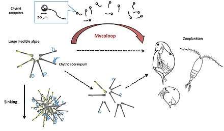
- Kagami, M., Miki, T. and Takimoto, G. (2014) "Mycoloop: chytrids in aquatic food webs". Frontiers in microbiology, 5: 166. doi:10.3389/fmicb.2014.00166.
- Gutierrez MH, Jara AM, Pantoja S (2016) "Fungal parasites infect marine diatoms in the upwelling ecosystem of the Humboldt current system off central Chile". Environ Microbiol, 18(5): 1646–1653. doi:10.1111/1462-2920.13257.
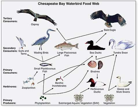
- US Geological Survey (USGS). "Chapter 14: Changes in Food and Habitats of Waterbirds." Figure 14.1. Synthesis of U.S. Geological Survey Science for the Chesapeake Bay Ecosystem and Implications for Environmental Management. USGS Circular 1316.

- Perry, M.C., Osenton, P.C., Wells-Berlin, A.M., and Kidwell, D.M., 2005, Food selection among Atlantic Coast sea ducks in relation to historic food habits, [abs.] in Perry, M.C., Second North American Sea Duck Conference, November 7–11, 2005, Annapolis, Maryland, Program and Abstracts, USGS Patuxent Wildlife Research Center, Maryland, 123 p. (p. 105).
- Bowser, A.K., Diamond, A.W. and Addison, J.A. (2013) "From puffins to plankton: a DNA-based analysis of a seabird food chain in the northern Gulf of Maine". PLoS One, 8(12): e83152. doi:10.1371/journal.pone.0083152
- Otero, X.L., De La Peña-Lastra, S., Pérez-Alberti, A., Ferreira, T.O. and Huerta-Diaz, M.A. (2018) "Seabird colonies as important global drivers in the nitrogen and phosphorus cycles". Nature communications, 9(1): 1–8. doi:10.1038/s41467-017-02446-8. Material was copied from this source, which is available under a Creative Commons Attribution 4.0 International License.
- Heymans, J.J., Coll, M., Libralato, S., Morissette, L. and Christensen, V. (2014). "Global patterns in ecological indicators of marine food webs: a modelling approach". PloS one, 9(4). doi:10.1371/journal.pone.0095845.
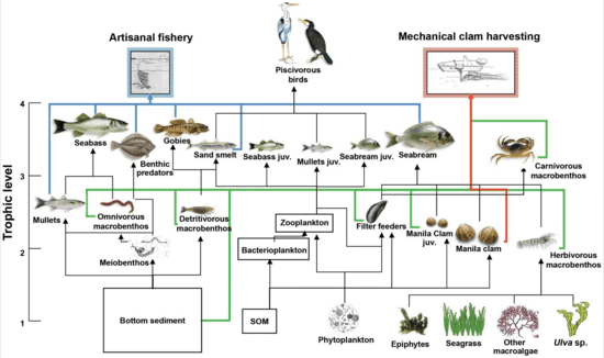
- Pranovi, F., Libralato, S., Raicevich, S., Granzotto, A., Pastres, R. and Giovanardi, O. (2003). "Mechanical clam dredging in Venice lagoon: ecosystem effects evaluated with a trophic mass-balance model". Marine Biology, 143(2): 393–403. doi:10.1007/s00227-003-1072-1.
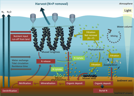
- Petersen, J.K., Holmer, M., Termansen, M. and Hasler, B. (2019) "Nutrient extraction through bivalves". In: Smaal A., Ferreira J., Grant J., Petersen J., Strand Ø. (eds) Goods and Services of Marine Bivalves, pages 179–208. Springer. doi:10.1007/978-3-319-96776-9_10. ISBN 9783319967769
- Coll, M., Schmidt, A., Romanuk, T. and Lotze, H.K. (2011). "Food-web structure of seagrass communities across different spatial scales and human impacts". PloS ONE, 6(7): e22591. doi:10.1371/journal.pone.0022591.
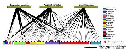
- Leray M, Meyer CP, Mills SC. (2015) "Metabarcoding dietary analysis of coral dwelling predatory fish demonstrates the minor contribution of coral mutualists to their highly partitioned, generalist diet". PeerJ, 3: e1047. doi:10.7717/peerj.1047.
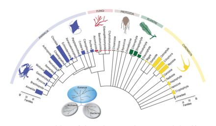
- Stat, M., Huggett, M.J., Bernasconi, R., DiBattista, J.D., Berry, T.E., Newman, S.J., Harvey, E.S. and Bunce, M. (2017) "Ecosystem biomonitoring with eDNA: metabarcoding across the tree of life in a tropical marine environment". Scientific Reports, 7(1): 1–11. doi:10.1038/s41598-017-12501-5.
- Lobo, Eduardo A.; Heinrich, Carla Giselda; Schuch, Marilia; Wetzel, Carlos Eduardo; Ector, Luc (2016), Necchi JR, Orlando (ed.), "Diatoms as Bioindicators in Rivers", River Algae, Springer International Publishing, pp. 245–271, doi:10.1007/978-3-319-31984-1_11, ISBN 9783319319834
- Stevenson, R. Jan; Pan, Yangdong; van Dam, Herman (2010), Smol, John P.; Stoermer, Eugene F. (eds.), "Assessing environmental conditions in rivers and streams with diatoms", The Diatoms (2 ed.), Cambridge University Press, pp. 57–85, doi:10.1017/cbo9780511763175.005, ISBN 9780511763175
- Kurata, N., Vella, K., Hamilton, B., Shivji, M., Soloviev, A., Matt, S., Tartar, A. and Perrie, W. (2016) "Surfactant-associated bacteria in the near-surface layer of the ocean". Nature: Scientific Reports, 6(1): 1–8. doi:10.1038/srep19123.
- Ẑutić, V., Ćosović, B., Marčenko, E., Bihari, N. and Kršinić, F. (1981) "Surfactant production by marine phytoplankton". Marine Chemistry, 10(6): 505–520. doi:10.1016/0304-4203(81)90004-9.
- Wang, F., Wu, Y., Chen, Z., Zhang, G., Zhang, J., Zheng, S. and Kattner, G. (2019) "Trophic interactions of mesopelagic fishes in the South China Sea illustrated by stable isotopes and fatty acids". Frontiers in Marine Science, 5: 522. doi:10.3389/fmars.2018.00522.
- Tollefson, Jeff (27 February 2020) Enter the twilight zone: scientists dive into the oceans’ mysterious middle Nature News. doi:10.1038/d41586-020-00520-8.
- Irigoien, X., Klevjer, T.A., Røstad, A., Martinez, U., Boyra, G., Acuña, J.L., Bode, A., Echevarria, F., Gonzalez-Gordillo, J.I., Hernandez-Leon, S. and Agusti, S. (2014) "Large mesopelagic fishes biomass and trophic efficiency in the open ocean". Nature communications, 5: 3271. doi:10.1038/ncomms4271
- Fish biomass in the ocean is 10 times higher than estimated EurekAlert, 7 February 2014.
- Choy, C.A., Haddock, S.H. and Robison, B.H. (2017) "Deep pelagic food web structure as revealed by in situ feeding observations". Proceedings of the Royal Society B: Biological Sciences, 284(1868): 20172116. doi:10.1098/rspb.2017.2116.
- Kelly, T.B., Davison, P.C., Goericke, R., Landry, M.R., Ohman, M. and Stukel, M.R. (2019) "The importance of mesozooplankton diel vertical migration for sustaining a mesopelagic food web". Frontiers in Marine Science, 6: 508. doi:10.3389/fmars.2019.00508.
- Choy, C.A., Wabnitz, C.C., Weijerman, M., Woodworth-Jefcoats, P.A. and Polovina, J.J. (2016) "Finding the way to the top: how the composition of oceanic mid-trophic micronekton groups determines apex predator biomass in the central North Pacific". Marine Ecology Progress Series, 549: 9–25. doi:10.3354/meps11680.
- Levin LA, Baco AR, Bowden DA, Colaco A, Cordes EE, Cunha MR, Demopoulos AWJ, Gobin J, Grupe BM, Le J, Metaxas A, Netburn AN, Rouse GW, Thurber AR, Tunnicliffe V, Van Dover CL, Vanreusel A and Watling L (2016). "Hydrothermal Vents and Methane Seeps: Rethinking the Sphere of Influence". Front. Mar. Sci. 3:72. doi:10.3389/fmars.2016.00072
- Portail, M., Olu, K., Dubois, S.F., Escobar-Briones, E., Gelinas, Y., Menot, L. and Sarrazin, J. (2016). "Food-web complexity in Guaymas Basin hydrothermal vents and cold seeps". PloS ONE, 11(9): p.e0162263. doi:10.1371/journal.pone.0162263.
- Bernardino AF, Levin LA, Thurber AR and Smith CR (2012). "Comparative Composition, Diversity and Trophic Ecology of Sediment Macrofauna at Vents, Seeps and Organic Falls". PLoS ONE, 7(4): e33515. pmid:22496753. doi:10.1371/journal.pone.0033515.
- Portail M, Olu K, Escobar-Briones E, Caprais JC, Menot L, Waeles M, et al. (2015). "Comparative study of vent and seep macrofaunal communities in the Guaymas Basin". Biogeosciences. 12(18): 5455–79. doi:10.5194/bg-12-5455-2015.
- Climate change in deep oceans could be seven times faster by middle of century, report says The Guardian, 25 May 2020.
- Brito-Morales, I., Schoeman, D.S., Molinos, J.G., Burrows, M.T., Klein, C.J., Arafeh-Dalmau, N., Kaschner, K., Garilao, C., Kesner-Reyes, K. and Richardson, A.J. (2020) "Climate velocity reveals increasing exposure of deep-ocean biodiversity to future warming". Nature Climate Change, pp.1-6. doi:10.5281/zenodo.3596584.
- McCarthy, J.J., Canziani, O.F., Leary, N.A., Dokken, D.J. and White, K.S. (Eds.) (2001) Climate Change 2001: Impacts, Adaptation, and Vulnerability: Contribution of Working Group II to the Third Assessment Report of the Intergovernmental Panel on Climate Change Page 807, Cambridge University Press. ISBN 9780521015004
- Murphy, E.J., Cavanagh, R.D., Drinkwater, K.F., Grant, S.M., Heymans, J.J., Hofmann, E.E., Hunt Jr, G.L. and Johnston, N.M. (2016) "Understanding the structure and functioning of polar pelagic ecosystems to predict the impacts of change". Proceedings of the Royal Society B: Biological Sciences, 283(1844): 20161646. doi:10.1098/rspb.2016.1646.
- Climate Impacts on Ecosystems: Food Web Disruptions EPA. Accessed 11 February 2020.
- Stoecker, D.K. and Lavrentyev, P.J. (2018). "Mixotrophic plankton in the polar seas: a pan-arctic review". Frontiers in Marine Science, 5: 292. doi:10.3389/fmars.2018.00292
- Bender, S.J., Moran, D.M., McIlvin, M.R., Zheng, H., McCrow, J.P., Badger, J., DiTullio, G.R., Allen, A.E. and Saito, M.A. (2018) "Colony formation in Phaeocystis antarctica: connecting molecular mechanisms with iron biogeochemistry". Biogeosciences, 15(16): 4923–4942. doi:10.5194/bg-15-4923-2018.
- Pinkernell, S. and Beszteri, B. (2014) "Potential effects of climate change on the distribution range of the main silicate sinker of the Southern Ocean". Ecology and evolution, 4(16): 3147–3161. doi:10.1002/ece3.1138
- Cavan, E.L., Belcher, A., Atkinson, A., Hill, S.L., Kawaguchi, S., McCormack, S., Meyer, B., Nicol, S., Ratnarajah, L., Schmidt, K. and Steinberg, D.K. (2019) "The importance of Antarctic krill in biogeochemical cycles". Nature communications, 10(1): 1–13. doi:10.1038/s41467-019-12668-7.
- Cordone, G., Marina, T.I., Salinas, V., Doyle, S.R., Saravia, L.A. and Momo, F.R.(2018). "Effects of macroalgae loss in an Antarctic marine food web: applying extinction thresholds to food web studies". PeerJ, 6: e5531. doi:10.7717/peerj.5531
- Marina, T.I., Salinas, V., Cordone, G., Campana, G., Moreira, E., Deregibus, D., Torre, L., Sahade, R., Tatian, M., Oro, E.B. and De Troch, M. (2018). "The food web of Potter Cove (Antarctica): complexity, structure and function". Estuarine, Coastal and Shelf Science, 200: 141–151. doi:10.1016/j.ecss.2017.10.015.
- Koh, E.Y., Martin, A.R., McMinn, A. and Ryan, K.G. (2012) "Recent advances and future perspectives in microbial phototrophy in Antarctic sea ice". Biology, 1(3): 542-556. doi:10.3390/biology1030542.
- The microbial loop here is re-drawn and abridged from:
- Azam, F., Fenchel, T., Field, J.G., Gray, J.S., Meyer-Reil, L.A. and Thingstad, F. (1983) "The ecological role of water-column microbes in the sea". Marine ecology progress series, 10(3): 257–263.
- Fenchel, T. (2008) "The microbial loop–25 years later". Journal of Experimental Marine Biology and Ecology, 366(1-2): 99-103. doi:10.1016/j.jembe.2008.07.013.
- Lamy, T., Koenigs, C., Holbrook, S.J., Miller, R.J., Stier, A.C. and Reed, D.C. (2020) "Foundation species promote community stability by increasing diversity in a giant kelp forest". Ecology, e02987. doi:10.1002/ecy.2987.
- Giant kelp gives Southern California marine ecosystems a strong foundation, National Science Foundation, 4 February 2020.
- Angelini, Christine; Altieri, Andrew H.; et al. (October 2011). "Interactions among Foundation Species and Their Consequences for Community Organization, Biodiversity, and Conservation". BioScience. 61 (10): 782–789. doi:10.1525/bio.2011.61.10.8.
- Ellison, Aaron M.; Bank, Michael S.; et al. (November 2005). "Loss of foundation species: consequences for the structure and dynamics of forested ecosystems". Frontiers in Ecology and the Environment. 3 (9): 479–486. doi:10.1890/1540-9295(2005)003[0479:LOFSCF]2.0.CO;2.
- Dayton, P. K. 1972. Toward an understanding of community resilience and the potential effects of enrichments to the benthos at McMurdo Sound, Antarctica. pp. 81–96 in Proceedings of the Colloquium on Conservation Problems Allen Press, Lawrence, Kansas.
- Paine, R. T. (1995). "A Conversation on Refining the Concept of Keystone Species". Conservation Biology. 9 (4): 962–964. doi:10.1046/j.1523-1739.1995.09040962.x.
- Davic, Robert D. (2003). "Linking Keystone Species and Functional Groups: A New Operational Definition of the Keystone Species Concept". Conservation Ecology. Retrieved 2011-02-03.
- Paine, R. T. (1969). "A Note on Trophic Complexity and Community Stability". The American Naturalist. 103 (929): 91–93. doi:10.1086/282586. JSTOR 2459472.
- "Keystone Species Hypothesis". University of Washington. Archived from the original on 2011-01-10. Retrieved 2011-02-03.
- Paine, R. T. (1966). "Food web complexity and species diversity". American Naturalist. 100 (910): 65–75. doi:10.1086/282400. JSTOR 2459379.
- Szpak, Paul; Orchard, Trevor J.; Salomon, Anne K.; Gröcke, Darren R. (2013). "Regional ecological variability and impact of the maritime fur trade on nearshore ecosystems in southern Haida Gwaii (British Columbia, Canada): evidence from stable isotope analysis of rockfish (Sebastes spp.) bone collagen". Archaeological and Anthropological Sciences. 5 (2): 159–182. doi:10.1007/s12520-013-0122-y.
- Cohn, J. P. (1998). "Understanding Sea Otters". BioScience. 48 (3): 151–155. doi:10.2307/1313259. JSTOR 1313259.
- Millette, N.C., Grosse, J., Johnson, W.M., Jungbluth, M.J. and Suter, E.A. (2018). "Hidden in plain sight: The importance of cryptic interactions in marine plankton". Limnology and Oceanography Letters, 3(4): 341–356. doi:10.1002/lol2.10084.
- Luypaert, T., Hagan, J.G., McCarthy, M.L. and Poti, M. (2020) "Status of Marine Biodiversity in the Anthropocene". In: YOUMARES 9-The Oceans: Our Research, Our Future, pages 57-82, Springer. doi:10.1007/978-3-030-20389-4_4.
- Estes JA, Tinker MT, Williams TM et al (1998) "Killer whale predation on sea otters linking oceanic and nearshore ecosystems". Science, 282: 473–476. doi:10.1126/science.282.5388.473.
- Post, D. M. (1993). "The long and short of food-chain length". Trends in Ecology and Evolution. 17 (6): 269–277. doi:10.1016/S0169-5347(02)02455-2.
- Jerry Bobrow, Ph.D.; Stephen Fisher (2009). CliffsNotes CSET: Multiple Subjects (2nd ed.). John Wiley and Sons. p. 283. ISBN 978-0-470-45546-3.
- Elton CS (1927) Animal Ecology. Republished 2001. University of Chicago Press.
- Paine RT (1966). "Food web complexity and species diversity". The American Naturalist. 100 (910): 65–75. doi:10.1086/282400.
- May RM (2001) Stability and Complexity in Model Ecosystems Princeton University Press, reprint of 1973 edition with new foreword. ISBN 978-0-691-08861-7.
- Pimm SL (2002) Food Webs University of Chicago Press, reprint of 1982 edition with new foreword. ISBN 978-0-226-66832-1.
- Kotta, J.; Wernberg, T.; Jänes, H.; Kotta, I.; Nurkse, K.; Pärnoja, M.; Orav-Kotta, H. (2018). "Novel crab predator causes marine ecosystem regime shift". Scientific Reports. 8 (1): 4956. doi:10.1038/s41598-018-23282-w. PMC 5897427. PMID 29651152.
- Megrey, Bernard and Werner, Francisco. "Evaluating the Role of Topdown vs. Bottom-up Ecosystem Regulation from a Modeling Perspective" (PDF).CS1 maint: multiple names: authors list (link)
- Frank, K. T.; Petrie, B.; Choi, J. S.; Leggett, W. C. (2005). "Trophic Cascades in a Formerly Cod-Dominated Ecosystem". Science. 308 (5728): 1621–1623. doi:10.1126/science.1113075. ISSN 0036-8075. PMID 15947186.
- Matsuzaki, Shin-Ichiro S.; Suzuki, Kenta; Kadoya, Taku; Nakagawa, Megumi; Takamura, Noriko (2018). "Bottom-up linkages between primary production, zooplankton, and fish in a shallow, hypereutrophic lake". Ecology. 99 (9): 2025–2036. doi:10.1002/ecy.2414. PMID 29884987.
- Lynam, Christopher Philip; Llope, Marcos; Möllmann, Christian; Helaouët, Pierre; Bayliss-Brown, Georgia Anne; Stenseth, Nils C. (Feb 2017). "Trophic and environmental control in the North Sea". Proceedings of the National Academy of Sciences. 114 (8): 1952–1957. doi:10.1073/pnas.1621037114. PMC 5338359. PMID 28167770.
- "Oldlist". Rocky Mountain Tree Ring Research. Retrieved January 8, 2013.
- Bar-On, Y.M., Phillips, R. and Milo, R. (2018) "The biomass distribution on Earth". Proceedings of the National Academy of Sciences, 115(25): 6506–6511. doi:10.1073/pnas.1711842115.
- Spellman, Frank R. (2008). The Science of Water: Concepts and Applications. CRC Press. p. 167. ISBN 978-1-4200-5544-3.
- Odum, E. P.; Barrett, G. W. (2005). Fundamentals of Ecology (5th ed.). Brooks/Cole, a part of Cengage Learning. ISBN 978-0-534-42066-6. Archived from the original on 2011-08-20.
- Wang, H.; Morrison, W.; Singh, A.; Weiss, H. (2009). "Modeling inverted biomass pyramids and refuges in ecosystems" (PDF). Ecological Modelling. 220 (11): 1376–1382. doi:10.1016/j.ecolmodel.2009.03.005. Archived from the original (PDF) on 2011-10-07.
- Field, C.B., Behrenfeld, M.J., Randerson, J.T. and Falkowski, P. (1998) "Primary production of the biosphere: integrating terrestrial and oceanic components". Science, 281(5374): 237–240. doi:10.1126/science.281.5374.237.
- Maureaud, A., Gascuel, D., Colléter, M., Palomares, M.L., Du Pontavice, H., Pauly, D. and Cheung, W.W. (2017) "Global change in the trophic functioning of marine food webs". PloS one, 12(8): e0182826. doi:10.1371/journal.pone.0182826
- "Effects of Ocean Acidification on Marine Species & Ecosystems". Report. OCEANA. Retrieved 13 October 2013.
- "Comprehensive study of Arctic Ocean acidification". Study. CICERO. Archived from the original on 10 December 2013. Retrieved 14 November 2013.
- Lischka, S.; Büdenbender J.; Boxhammer T.; Riebesell U. (15 April 2011). "Impact of ocean acidification and elevated temperatures on early juveniles of the polar shelled pteropod Limacina helicina : mortality, shell degradation, and shell growth" (PDF). Report. Biogeosciences. pp. 919–932. Retrieved 14 November 2013.
- "Antarctic marine wildlife is under threat, study finds". BBC Nature. Retrieved 13 October 2013.
- Ullah, H., Nagelkerken, I., Goldenberg, S.U. and Fordham, D.A. (2018) "Climate change could drive marine food web collapse through altered trophic flows and cyanobacterial proliferation". PLoS biology, 16(1): e2003446. doi:10.1371/journal.pbio.2003446
- Climate change drives collapse in marine food webs ScienceDaily. 9 January 2018.
- IUCN (2018) The IUCN Red List of Threatened Species: Version 2018-1