Diffusion
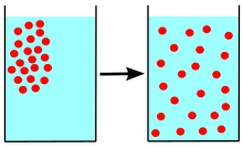
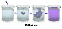
Diffusion is the net movement of molecules or atoms from a region of high concentration (or high chemical potential) to a region of low concentration (or low chemical potential) as a result of random motion of the molecules or atoms. Diffusion is driven by a gradient in chemical potential of the diffusing species.
A gradient is the change in the value of a quantity e.g. concentration, pressure, or temperature with the change in another variable, usually distance. A change in concentration over a distance is called a concentration gradient, a change in pressure over a distance is called a pressure gradient, and a change in temperature over a distance is called a temperature gradient.
The word diffusion derives from the Latin word, diffundere, which means "to spread way out".
A distinguishing feature of diffusion is that it depends on particle random walk, and results in mixing or mass transport without requiring directed bulk motion. Bulk motion, or bulk flow, is the characteristic of advection.[1] The term convection is used to describe the combination of both transport phenomena.
Diffusion vs. bulk flow
An example of a situation in which bulk motion and diffusion can be differentiated is the mechanism by which oxygen enters the body during external respiration known as breathing. The lungs are located in the thoracic cavity, which expands as the first step in external respiration. This expansion leads to an increase in volume of the alveoli in the lungs, which causes a decrease in pressure in the alveoli. This creates a pressure gradient between the air outside the body at relatively high pressure and the alveoli at relatively low pressure. The air moves down the pressure gradient through the airways of the lungs and into the alveoli until the pressure of the air and that in the alveoli are equal i.e. the movement of air by bulk flow stops once there is no longer a pressure gradient.
The air arriving in the alveoli has a higher concentration of oxygen than the “stale” air in the alveoli. The increase in oxygen concentration creates a concentration gradient for oxygen between the air in the alveoli and the blood in the capillaries that surround the alveoli. Oxygen then moves by diffusion, down the concentration gradient, into the blood. The other consequence of the air arriving in alveoli is that the concentration of carbon dioxide in the alveoli decreases. This creates a concentration gradient for carbon dioxide to diffuse from the blood into the alveoli, as fresh air has a very low concentration of carbon dioxide compared to the blood in the body.
The pumping action of the heart then transports the blood around the body. As the left ventricle of the heart contracts, the volume decreases, which increases the pressure in the ventricle. This creates a pressure gradient between the heart and the capillaries, and blood moves through blood vessels by bulk flow down the pressure gradient. As the thoracic cavity contracts during expiration, the volume of the alveoli decreases and creates a pressure gradient between the alveoli and the air outside the body, and air moves by bulk flow down the pressure gradient.
Diffusion in the context of different disciplines

The concept of diffusion is widely used in: physics (particle diffusion), chemistry, biology, sociology, economics, and finance (diffusion of people, ideas and of price values). However, in each case, the object (e.g., atom, idea, etc.) that is undergoing diffusion is “spreading out” from a point or location at which there is a higher concentration of that object.
There are two ways to introduce the notion of diffusion: either a phenomenological approach starting with Fick's laws of diffusion and their mathematical consequences, or a physical and atomistic one, by considering the random walk of the diffusing particles.[2]
In the phenomenological approach, diffusion is the movement of a substance from a region of high concentration to a region of low concentration without bulk motion. According to Fick's laws, the diffusion flux is proportional to the negative gradient of concentrations. It goes from regions of higher concentration to regions of lower concentration. Sometime later, various generalizations of Fick's laws were developed in the frame of thermodynamics and non-equilibrium thermodynamics.[3]
From the atomistic point of view, diffusion is considered as a result of the random walk of the diffusing particles. In molecular diffusion, the moving molecules are self-propelled by thermal energy. Random walk of small particles in suspension in a fluid was discovered in 1827 by Robert Brown. The theory of the Brownian motion and the atomistic backgrounds of diffusion were developed by Albert Einstein.[4] The concept of diffusion is typically applied to any subject matter involving random walks in ensembles of individuals.
Biologists often use the terms "net movement" or "net diffusion" to describe the movement of ions or molecules by diffusion. For example, oxygen can diffuse through cell membranes so long as there is a higher concentration of oxygen outside the cell. However, because the movement of molecules is random, occasionally oxygen molecules move out of the cell (against the concentration gradient). Because there are more oxygen molecules outside the cell, the probability that oxygen molecules will enter the cell is higher than the probability that oxygen molecules will leave the cell. Therefore, the "net" movement of oxygen molecules (the difference between the number of molecules either entering or leaving the cell) is into the cell. In other words, there is a net movement of oxygen molecules down the concentration gradient.
History of diffusion in physics
In the scope of time, diffusion in solids was used long before the theory of diffusion was created. For example, Pliny the Elder had previously described the cementation process, which produces steel from the element iron (Fe) through carbon diffusion. Another example is well known for many centuries, the diffusion of colors of stained glass or earthenware and Chinese ceramics.
In modern science, the first systematic experimental study of diffusion was performed by Thomas Graham. He studied diffusion in gases, and the main phenomenon was described by him in 1831–1833:[5]
"...gases of different nature, when brought into contact, do not arrange themselves according to their density, the heaviest undermost, and the lighter uppermost, but they spontaneously diffuse, mutually and equally, through each other, and so remain in the intimate state of mixture for any length of time.”
The measurements of Graham contributed to James Clerk Maxwell deriving, in 1867, the coefficient of diffusion for CO2 in the air. The error rate is less than 5%.
In 1855, Adolf Fick, the 26-year-old anatomy demonstrator from Zürich, proposed his law of diffusion. He used Graham's research, stating his goal as "the development of a fundamental law, for the operation of diffusion in a single element of space". He asserted a deep analogy between diffusion and conduction of heat or electricity, creating a formalism that is similar to Fourier's law for heat conduction (1822) and Ohm's law for electric current (1827).
Robert Boyle demonstrated diffusion in solids in the 17th century[6] by penetration of zinc into a copper coin. Nevertheless, diffusion in solids was not systematically studied until the second part of the 19th century. William Chandler Roberts-Austen, the well-known British metallurgist and former assistant of Thomas Graham studied systematically solid state diffusion on the example of gold in lead in 1896. :[7]
"... My long connection with Graham's researches made it almost a duty to attempt to extend his work on liquid diffusion to metals."
In 1858, Rudolf Clausius introduced the concept of the mean free path. In the same year, James Clerk Maxwell developed the first atomistic theory of transport processes in gases. The modern atomistic theory of diffusion and Brownian motion was developed by Albert Einstein, Marian Smoluchowski and Jean-Baptiste Perrin. Ludwig Boltzmann, in the development of the atomistic backgrounds of the macroscopic transport processes, introduced the Boltzmann equation, which has served mathematics and physics with a source of transport process ideas and concerns for more than 140 years.[8]
In 1920–1921, George de Hevesy measured self-diffusion using radioisotopes. He studied self-diffusion of radioactive isotopes of lead in the liquid and solid lead.
Yakov Frenkel (sometimes, Jakov/Jacob Frenkel) proposed, and elaborated in 1926, the idea of diffusion in crystals through local defects (vacancies and interstitial atoms). He concluded, the diffusion process in condensed matter is an ensemble of elementary jumps and quasichemical interactions of particles and defects. He introduced several mechanisms of diffusion and found rate constants from experimental data.
Sometime later, Carl Wagner and Walter H. Schottky developed Frenkel's ideas about mechanisms of diffusion further. Presently, it is universally recognized that atomic defects are necessary to mediate diffusion in crystals.[7]
Henry Eyring, with co-authors, applied his theory of absolute reaction rates to Frenkel's quasichemical model of diffusion.[9] The analogy between reaction kinetics and diffusion leads to various nonlinear versions of Fick's law.[10]
Basic models of diffusion
Diffusion flux
Each model of diffusion expresses the diffusion flux through concentrations, densities and their derivatives. Flux is a vector . The transfer of a physical quantity through a small area with normal per time is


where is the inner product and is the little-o notation. If we use the notation of vector area then


The dimension of the diffusion flux is [flux] = [quantity]/([time]·[area]). The diffusing physical quantity may be the number of particles, mass, energy, electric charge, or any other scalar extensive quantity. For its density, , the diffusion equation has the form


where is intensity of any local source of this quantity (the rate of a chemical reaction, for example). For the diffusion equation, the no-flux boundary conditions can be formulated as on the boundary, where is the normal to the boundary at point .


Fick's law and equations
Fick's first law: the diffusion flux is proportional to the negative of the concentration gradient:

The corresponding diffusion equation (Fick's second law) is

where is the Laplace operator,


Onsager's equations for multicomponent diffusion and thermodiffusion
Fick's law describes diffusion of an admixture in a medium. The concentration of this admixture should be small and the gradient of this concentration should be also small. The driving force of diffusion in Fick's law is the antigradient of concentration, .

In 1931, Lars Onsager[11] included the multicomponent transport processes in the general context of linear non-equilibrium thermodynamics. For multi-component transport,

where is the flux of the ith physical quantity (component) and is the jth thermodynamic force.


The thermodynamic forces for the transport processes were introduced by Onsager as the space gradients of the derivatives of the entropy density s (he used the term "force" in quotation marks or "driving force"):

where are the "thermodynamic coordinates". For the heat and mass transfer one can take (the density of internal energy) and is the concentration of the ith component. The corresponding driving forces are the space vectors


- because


where T is the absolute temperature and is the chemical potential of the ith component. It should be stressed that the separate diffusion equations describe the mixing or mass transport without bulk motion. Therefore, the terms with variation of the total pressure are neglected. It is possible for diffusion of small admixtures and for small gradients.

For the linear Onsager equations, we must take the thermodynamic forces in the linear approximation near equilibrium:

where the derivatives of s are calculated at equilibrium n*. The matrix of the kinetic coefficients should be symmetric (Onsager reciprocal relations) and positive definite (for the entropy growth).

The transport equations are
![{\displaystyle {\frac {\partial n_{i}}{\partial t}}=-\operatorname {div} \mathbf {J} _{i}=-\sum _{j\geq 0}L_{ij}\operatorname {div} X_{j}=\sum _{k\geq 0}\left[-\sum _{j\geq 0}L_{ij}\left.{\frac {\partial ^{2}s(n)}{\partial n_{j}\,\partial n_{k}}}\right|_{n=n^{*}}\right]\,\Delta n_{k}\ .}](../I/m/f61d376b495038f57128d2c6ea83f733b7ae0b83.svg)
Here, all the indexes i, j, k = 0, 1, 2, ... are related to the internal energy (0) and various components. The expression in the square brackets is the matrix of the diffusion (i,k > 0), thermodiffusion (i > 0, k = 0 or k > 0, i = 0) and thermal conductivity (i = k = 0) coefficients.

Under isothermal conditions T = constant. The relevant thermodynamic potential is the free energy (or the free entropy). The thermodynamic driving forces for the isothermal diffusion are antigradients of chemical potentials, , and the matrix of diffusion coefficients is


(i,k > 0).
There is intrinsic arbitrariness in the definition of the thermodynamic forces and kinetic coefficients because they are not measurable separately and only their combinations can be measured. For example, in the original work of Onsager[11] the thermodynamic forces include additional multiplier T, whereas in the Course of Theoretical Physics[12] this multiplier is omitted but the sign of the thermodynamic forces is opposite. All these changes are supplemented by the corresponding changes in the coefficients and do not affect the measurable quantities.

Nondiagonal diffusion must be nonlinear
The formalism of linear irreversible thermodynamics (Onsager) generates the systems of linear diffusion equations in the form

If the matrix of diffusion coefficients is diagonal, then this system of equations is just a collection of decoupled Fick's equations for various components. Assume that diffusion is non-diagonal, for example, , and consider the state with . At this state, . If at some points, then becomes negative at these points in a short time. Therefore, linear non-diagonal diffusion does not preserve positivity of concentrations. Non-diagonal equations of multicomponent diffusion must be non-linear.[10]


Einstein's mobility and Teorell formula
The Einstein relation (kinetic theory) connects the diffusion coefficient and the mobility (the ratio of the particle's terminal drift velocity to an applied force)[13]

where D is the diffusion constant, μ is the "mobility", kB is Boltzmann's constant, T is the absolute temperature.
Below, to combine in the same formula the chemical potential μ and the mobility, we use for mobility the notation .

The mobility—based approach was further applied by T. Teorell.[14] In 1935, he studied the diffusion of ions through a membrane. He formulated the essence of his approach in the formula:
- the flux is equal to mobility × concentration × force per gram-ion.
This is the so-called Teorell formula. The term "gram-ion" ("gram-particle") is used for a quantity of a substance that contains Avogadro's number of ions (particles). The common modern term is mole.
The force under isothermal conditions consists of two parts:
- Diffusion force caused by concentration gradient: .
- Electrostatic force caused by electric potential gradient: .


Here R is the gas constant, T is the absolute temperature, n is the concentration, the equilibrium concentration is marked by a superscript "eq", q is the charge and φ is the electric potential.
The simple but crucial difference between the Teorell formula and the Onsager laws is the concentration factor in the Teorell expression for the flux. In the Einstein–Teorell approach, If for the finite force the concentration tends to zero then the flux also tends to zero, whereas the Onsager equations violate this simple and physically obvious rule.
The general formulation of the Teorell formula for non-perfect systems under isothermal conditions is[10]

where μ is the chemical potential, μ0 is the standard value of the chemical potential. The expression is the so-called activity. It measures the "effective concentration" of a species in a non-ideal mixture. In this notation, the Teorell formula for the flux has a very simple form[10]


The standard derivation of the activity includes a normalization factor and for small concentrations , where is the standard concentration. Therefore, this formula for the flux describes the flux of the normalized dimensionless quantity :


![{\displaystyle {\frac {\partial (n/n^{\ominus })}{\partial t}}=\nabla \cdot [{\mathfrak {m}}a(\nabla \mu -({\text{external force per mole}}))].}](../I/m/3f8ae11dd009457b8fd39d1a583ed5d4b3e30ab5.svg)
Teorell formula for multicomponent diffusion
The Teorell formula with combination of Onsager's definition of the diffusion force gives

where is the mobility of the ith component, is its activity, is the matrix of the coefficients, is the thermodynamic diffusion force, . For the isothermal perfect systems, . Therefore, the Einstein–Teorell approach gives the following multicomponent generalization of the Fick's law for multicomponent diffusion:


where is the matrix of coefficients. The Chapman–Enskog formulas for diffusion in gases include exactly the same terms. Earlier, such terms were introduced in the Maxwell–Stefan diffusion equation.

Jumps on the surface and in solids
Diffusion of reagents on the surface of a catalyst may play an important role in heterogeneous catalysis. The model of diffusion in the ideal monolayer is based on the jumps of the reagents on the nearest free places. This model was used for CO on Pt oxidation under low gas pressure.
The system includes several reagents on the surface. Their surface concentrations are The surface is a lattice of the adsorption places. Each reagent molecule fills a place on the surface. Some of the places are free. The concentration of the free places is . The sum of all (including free places) is constant, the density of adsorption places b.


The jump model gives for the diffusion flux of (i = 1, ..., n):

![{\displaystyle \mathbf {J} _{i}=-D_{i}[z\,\nabla c_{i}-c_{i}\nabla z]\,.}](../I/m/e62d2876591f6c0c24854dc77bd002742a487757.svg)
The corresponding diffusion equation is:[10]
![{\displaystyle {\frac {\partial c_{i}}{\partial t}}=-\operatorname {div} \mathbf {J} _{i}=D_{i}[z\,\Delta c_{i}-c_{i}\,\Delta z]\,.}](../I/m/59acf7a4d07ec81e21aec16a7dd999c091b60b79.svg)
Due to the conservation law, and we have the system of m diffusion equations. For one component we get Fick's law and linear equations because . For two and more components the equations are nonlinear.


If all particles can exchange their positions with their closest neighbours then a simple generalization gives
![{\displaystyle \mathbf {J} _{i}=-\sum _{j}D_{ij}[c_{j}\,\nabla c_{i}-c_{i}\,\nabla c_{j}]}](../I/m/aba83bc12bd5bab3419c70e17305975783df881d.svg)
![{\displaystyle {\frac {\partial c_{i}}{\partial t}}=\sum _{j}D_{ij}[c_{j}\,\Delta c_{i}-c_{i}\,\Delta c_{j}]}](../I/m/63b9c514f4d2f44400b6315598831cacc5edaee9.svg)
where is a symmetric matrix of coefficients that characterize the intensities of jumps. The free places (vacancies) should be considered as special "particles" with concentration .


Various versions of these jump models are also suitable for simple diffusion mechanisms in solids.
Diffusion in porous media
For diffusion in porous media the basic equations are:[15]


where D is the diffusion coefficient, n is the concentration, m > 0 (usually m > 1, the case m = 1 corresponds to Fick's law).
For diffusion of gases in porous media this equation is the formalisation of Darcy's law: the velocity of a gas in the porous media is

where k is the permeability of the medium, μ is the viscosity and p is the pressure. The flux J = nv and for Darcy's law gives the equation of diffusion in porous media with m = γ + 1.

For underground water infiltration, the Boussinesq approximation gives the same equation with m = 2.
For plasma with the high level of radiation, the Zeldovich–Raizer equation gives m > 4 for the heat transfer.
Diffusion in physics
Elementary theory of diffusion coefficient in gases
The diffusion coefficient is the coefficient in the Fick's first law , where J is the diffusion flux (amount of substance) per unit area per unit time, n (for ideal mixtures) is the concentration, x is the position [length].


Let us consider two gases with molecules of the same diameter d and mass m (self-diffusion). In this case, the elementary mean free path theory of diffusion gives for the diffusion coefficient

where kB is the Boltzmann constant, T is the temperature, P is the pressure, is the mean free path, and vT is the mean thermal speed:


We can see that the diffusion coefficient in the mean free path approximation grows with T as T3/2 and decreases with P as 1/P. If we use for P the ideal gas law P = RnT with the total concentration n, then we can see that for given concentration n the diffusion coefficient grows with T as T1/2 and for given temperature it decreases with the total concentration as 1/n.
For two different gases, A and B, with molecular masses mA, mB and molecular diameters dA, dB, the mean free path estimate of the diffusion coefficient of A in B and B in A is:

The theory of diffusion in gases based on Boltzmann's equation
In Boltzmann's kinetics of the mixture of gases, each gas has its own distribution function, , where t is the time moment, x is position and c is velocity of molecule of the ith component of the mixture. Each component has its mean velocity . If the velocities do not coincide then there exists diffusion.


In the Chapman–Enskog approximation, all the distribution functions are expressed through the densities of the conserved quantities:[8]
- individual concentrations of particles, (particles per volume),
- density of momentum (mi is the ith particle mass),
- density of kinetic energy


The kinetic temperature T and pressure P are defined in 3D space as

where is the total density.

For two gases, the difference between velocities, is given by the expression:[8]


where is the force applied to the molecules of the ith component and is the thermodiffusion ratio.


The coefficient D12 is positive. This is the diffusion coefficient. Four terms in the formula for C1-C2 describe four main effects in the diffusion of gases:
- describes the flux of the first component from the areas with the high ratio n1/n to the areas with lower values of this ratio (and, analogously the flux of the second component from high n2/n to low n2/n because n2/n = 1 – n1/n);
- describes the flux of the heavier molecules to the areas with higher pressure and the lighter molecules to the areas with lower pressure, this is barodiffusion;
- describes diffusion caused by the difference of the forces applied to molecules of different types. For example, in the Earth's gravitational field, the heavier molecules should go down, or in electric field the charged molecules should move, until this effect is not equilibrated by the sum of other terms. This effect should not be confused with barodiffusion caused by the pressure gradient.
- describes thermodiffusion, the diffusion flux caused by the temperature gradient.


All these effects are called diffusion because they describe the differences between velocities of different components in the mixture. Therefore, these effects cannot be described as a bulk transport and differ from advection or convection.
In the first approximation,[8]
- for rigid spheres;
- for repulsing force
![{\displaystyle D_{12}={\frac {3}{2n(d_{1}+d_{2})^{2}}}\left[{\frac {kT(m_{1}+m_{2})}{2\pi m_{1}m_{2}}}\right]^{1/2}}](../I/m/0f17effad1f63d0da95fb3082d73481f845e1785.svg)
![{\displaystyle D_{12}={\frac {3}{8nA_{1}({\nu })\Gamma (3-{\frac {2}{\nu -1}})}}\left[{\frac {kT(m_{1}+m_{2})}{2\pi m_{1}m_{2}}}\right]^{1/2}\left({\frac {2kT}{\kappa _{12}}}\right)^{\frac {2}{\nu -1}}}](../I/m/a21bffa231a21e8104224bb96f51c7a59685b908.svg)

The number is defined by quadratures (formulas (3.7), (3.9), Ch. 10 of the classical Chapman and Cowling book[8])

We can see that the dependence on T for the rigid spheres is the same as for the simple mean free path theory but for the power repulsion laws the exponent is different. Dependence on a total concentration n for a given temperature has always the same character, 1/n.
In applications to gas dynamics, the diffusion flux and the bulk flow should be joined in one system of transport equations. The bulk flow describes the mass transfer. Its velocity V is the mass average velocity. It is defined through the momentum density and the mass concentrations:

where is the mass concentration of the ith species, is the mass density.


By definition, the diffusion velocity of the ith component is , . The mass transfer of the ith component is described by the continuity equation


where is the net mass production rate in chemical reactions, .


In these equations, the term describes advection of the ith component and the term represents diffusion of this component.


In 1948, Wendell H. Furry proposed to use the form of the diffusion rates found in kinetic theory as a framework for the new phenomenological approach to diffusion in gases. This approach was developed further by F.A. Williams and S.H. Lam.[16] For the diffusion velocities in multicomponent gases (N components) they used


Here, is the diffusion coefficient matrix, is the thermal diffusion coefficient, is the body force per unite mass acting on the ith species, is the partial pressure fraction of the ith species (and is the partial pressure), is the mass fraction of the ith species, and


Diffusion of electrons in solids
When the density of electrons in solids is not in equilibrium, diffusion of electrons occurs. For example, when a bias is applied to two ends of a chunk of semiconductor, or a light shines on one end (see right figure), electron diffuse from high density regions (center) to low density regions (two ends), forming a gradient of electron density. This process generates current, referred to as diffusion current.
Diffusion current can also be described by Fick's first law

where J is the diffusion current density (amount of substance) per unit area per unit time, n (for ideal mixtures) is the electron density, x is the position [length].
Diffusion in geophysics
Analytical and numerical models that solve the diffusion equation for different initial and boundary conditions have been popular for studying a wide variety of changes to the Earth's surface. Diffusion has been used extensively in erosion studies of hillslope retreat, bluff erosion, fault scarp degradation, wave-cut terrace/shoreline retreat, alluvial channel incision, coastal shelf retreat, and delta progradation[17]. Although the Earth's surface is not literally diffusing in many of these cases, the process of diffusion effectively mimics the holistic changes that occur over decades to millennia. Diffusion models may also be used to solve inverse boundary value problems in which some information about the depositional environment is known from paleoenvironmental reconstruction and the diffusion equation is used to figure out the sediment influx and time series of landform changes[18].
Random walk (random motion)
One common misconception is that individual atoms, ions or molecules move randomly, which they do not. In the animation on the right, the ion on in the left panel has a “random” motion, but this motion is not random as it is the result of “collisions” with other ions. As such, the movement of a single atom, ion, or molecule within a mixture just appears random when viewed in isolation. The movement of a substance within a mixture by “random walk” is governed by the kinetic energy within the system that can be affected by changes in concentration, pressure or temperature.
Separation of diffusion from convection in gases
While Brownian motion of multi-molecular mesoscopic particles (like pollen grains studied by Brown) is observable under an optical microscope, molecular diffusion can only be probed in carefully controlled experimental conditions. Since Graham experiments, it is well known that avoiding of convection is necessary and this may be a non-trivial task.
Under normal conditions, molecular diffusion dominates only on length scales between nanometer and millimeter. On larger length scales, transport in liquids and gases is normally due to another transport phenomenon, convection, and to study diffusion on the larger scale, special efforts are needed.
Therefore, some often cited examples of diffusion are wrong: If cologne is sprayed in one place, it can soon be smelled in the entire room, but a simple calculation shows that this can't be due to diffusion. Convective motion persists in the room because of the temperature [inhomogeneity]. If ink is dropped in water, one usually observes an inhomogeneous evolution of the spatial distribution, which clearly indicates convection (caused, in particular, by this dropping).
In contrast, heat conduction through solid media is an everyday occurrence (e.g. a metal spoon partly immersed in a hot liquid). This explains why the diffusion of heat was explained mathematically before the diffusion of mass.
Other types of diffusion
- Anisotropic diffusion, also known as the Perona–Malik equation, enhances high gradients
- Anomalous diffusion,[19] in porous medium
- Atomic diffusion, in solids
- Eddy diffusion, in coarse-grained description of turbulent flow
- Effusion of a gas through small holes
- Electronic diffusion, resulting in an electric current called the diffusion current
- Facilitated diffusion, present in some organisms
- Gaseous diffusion, used for isotope separation
- Heat equation, diffusion of thermal energy
- Itō diffusion, mathematisation of Brownian motion, continuous stochastic process.
- Kinesis (biology) is an animal's non-directional movement activity in response to a stimulus.
- Knudsen diffusion of gas in long pores with frequent wall collisions
- Levy flights and walks
- Momentum diffusion ex. the diffusion of the hydrodynamic velocity field
- Photon diffusion
- Plasma diffusion
- Random walk,[20] model for diffusion
- Reverse diffusion, against the concentration gradient, in phase separation
- Rotational diffusion, random reorientations of molecules
- Surface diffusion, diffusion of adparticles on a surface
- Turbulent diffusion, transport of mass, heat, or momentum within a turbulent fluid
See also
References
- ↑ J.G. Kirkwood, R.L. Baldwin, P.J. Dunlop, L.J. Gosting, G. Kegeles (1960)Flow equations and frames of reference for isothermal diffusion in liquids. The Journal of Chemical Physics 33(5):1505–13.
- ↑ J. Philibert (2005). One and a half century of diffusion: Fick, Einstein, before and beyond. Archived 2013-12-13 at the Wayback Machine. Diffusion Fundamentals, 2, 1.1–1.10.
- ↑ S.R. De Groot, P. Mazur (1962). Non-equilibrium Thermodynamics. North-Holland, Amsterdam.
- ↑ A. Einstein (1905). "Über die von der molekularkinetischen Theorie der Wärme geforderte Bewegung von in ruhenden Flüssigkeiten suspendierten Teilchen" (PDF). Ann. Phys. 17 (8): 549–60. Bibcode:1905AnP...322..549E. doi:10.1002/andp.19053220806.
- ↑ Diffusion Processes, Thomas Graham Symposium, ed. J.N. Sherwood, A.V. Chadwick, W.M.Muir, F.L. Swinton, Gordon and Breach, London, 1971.
- ↑ L.W. Barr (1997), In: Diffusion in Materials, DIMAT 96, ed. H.Mehrer, Chr. Herzig, N.A. Stolwijk, H. Bracht, Scitec Publications, Vol.1, pp. 1–9.
- 1 2 H. Mehrer; N.A. Stolwijk (2009). "Heroes and Highlights in the History of Diffusion" (PDF). Diffusion Fundamentals. 11 (1): 1–32.
- 1 2 3 4 5 S. Chapman, T. G. Cowling (1970) The Mathematical Theory of Non-uniform Gases: An Account of the Kinetic Theory of Viscosity, Thermal Conduction and Diffusion in Gases, Cambridge University Press (3rd edition), ISBN 052140844X.
- ↑ J.F. Kincaid; H. Eyring; A.E. Stearn (1941). "The theory of absolute reaction rates and its application to viscosity and diffusion in the liquid State". Chem. Rev. 28 (2): 301–65. doi:10.1021/cr60090a005.
- 1 2 3 4 5 A.N. Gorban, H.P. Sargsyan and H.A. Wahab (2011). "Quasichemical Models of Multicomponent Nonlinear Diffusion". Mathematical Modelling of Natural Phenomena. 6 (5): 184–262. arXiv:1012.2908. doi:10.1051/mmnp/20116509.
- 1 2 Onsager, L. (1931). "Reciprocal Relations in Irreversible Processes. I". Physical Review. 37 (4): 405–26. Bibcode:1931PhRv...37..405O. doi:10.1103/PhysRev.37.405.
- ↑ L.D. Landau, E.M. Lifshitz (1980). Statistical Physics. Vol. 5 (3rd ed.). Butterworth-Heinemann. ISBN 978-0-7506-3372-7.
- ↑ S. Bromberg, K.A. Dill (2002), Molecular Driving Forces: Statistical Thermodynamics in Chemistry and Biology, Garland Science, ISBN 0815320515.
- ↑ T. Teorell (1935). "Studies on the "Diffusion Effect" upon Ionic Distribution. Some Theoretical Considerations". Proceedings of the National Academy of Sciences of the United States of America. 21 (3): 152–61. Bibcode:1935PNAS...21..152T. doi:10.1073/pnas.21.3.152. PMC 1076553. PMID 16587950.
- ↑ J. L. Vázquez (2006), The Porous Medium Equation. Mathematical Theory, Oxford Univ. Press, ISBN 0198569033.
- ↑ S. H. Lam (2006). "Multicomponent diffusion revisited" (PDF). Physics of Fluids. 18 (7): 073101. Bibcode:2006PhFl...18g3101L. doi:10.1063/1.2221312.
- ↑ Pasternack, Gregory B.; Brush, Grace S.; Hilgartner, William B. (2001-04-01). "Impact of historic land-use change on sediment delivery to a Chesapeake Bay subestuarine delta". Earth Surface Processes and Landforms. 26 (4): 409–27. Bibcode:2001ESPL...26..409P. doi:10.1002/esp.189. ISSN 1096-9837.
- ↑ Gregory B. Pasternack. "Watershed Hydrology, Geomorphology, and Ecohydraulics :: TFD Modeling". pasternack.ucdavis.edu. Retrieved 2017-06-12.
- ↑ D. Ben-Avraham and S. Havlin (2000). Diffusion and Reactions in Fractals and Disordered Systems (PDF). Cambridge University Press. ISBN 0521622786.
- ↑ Weiss, G. (1994). Aspects and Applications of the Random Walk. North-Holland. ISBN 0444816062.