Viscosity

Viscosity
	A simulation of liquids with different viscosities. The liquid on the right has higher viscosity than the liquid on the left.
Common symbols	η, μ
Derivations from; other quantities	μ = G·t

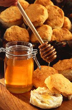
The viscosity of a fluid is the measure of its resistance to gradual deformation by shear stress or tensile stress.^[1] For liquids, it corresponds to the informal concept of "thickness": for example, honey has a higher viscosity than water.^[2]

Viscosity is the property of a fluid which opposes the relative motion between two surfaces of the fluid that are moving at different velocities. In simple terms, viscosity means friction between the molecules of fluid. When the fluid is forced through a tube, the particles which compose the fluid generally move more quickly near the tube's axis and more slowly near its walls; therefore some stress (such as a pressure difference between the two ends of the tube) is needed to overcome the friction between particle layers to keep the fluid moving. For a given velocity pattern, the stress required is proportional to the fluid's viscosity.

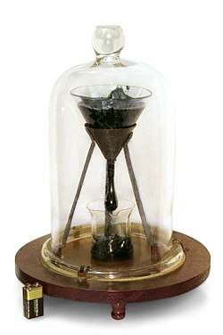
A fluid that has no resistance to shear stress is known as an ideal or inviscid fluid. Zero viscosity is observed only at very low temperatures in superfluids. Otherwise, all fluids have positive viscosity and are technically said to be viscous or viscid. A fluid with a relatively high viscosity, such as pitch, may appear to be a solid.

Etymology

The word "viscosity" is derived from the Latin "viscum", meaning mistletoe and also a viscous glue made from mistletoe berries.^[3]

Definition

Simple definition

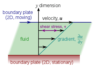
Illustration of a planar Couette flow. Since the shearing flow is opposed by friction between adjacent layers of fluid (which are in relative motion), a force is required to sustain the motion of the upper plate. The relative strength of this force is a measure of the fluid's viscosity.

In a general parallel flow, the shear stress is proportional to the gradient of the velocity.

The viscosity of a fluid expresses its resistance to shearing flows, in which adjacent fluid layers are in relative motion. A simple example of such a shearing flow is a planar Couette flow, where a fluid is trapped between two infinitely large plates, one fixed and one in parallel motion at constant speed $u$ (see illustration to the right). Although viscosity applies to general flows, it is easy to define and visualize in a Couette flow.

If the speed of the top plate is low enough, then in steady state the fluid particles move parallel to it, and their speed varies from $0$ at the bottom to $u$ at the top. Each layer of fluid moves faster than the one just below it, and friction between them gives rise to a force resisting their relative motion. In particular, the fluid applies on the top plate a force in the direction opposite to its motion, and an equal but opposite force on the bottom plate. An external force is therefore required in order to keep the top plate moving at constant speed.

In many fluids, the flow velocity is observed to vary linearly from zero at the bottom to $u$ at the top. Moreover, the magnitude $F$ of the force acting on the top plate is found to be proportional to the speed $u$ and the area $A$ of each plate, and inversely proportional to their separation $y$ :

F=\mu A{\frac {u}{y}}.

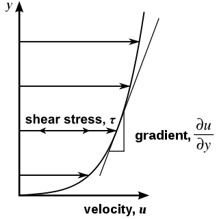
The proportionality factor $μ$ is the viscosity of the fluid, with units of ${\text{Pa}}\cdot {\text{s}}$ (pascal-second). The ratio $u / y$ is called the rate of shear deformation or shear velocity, and is the derivative of the fluid speed in the direction perpendicular to the plates (see illustrations to the right). If the velocity does not vary linearly with $y$ , then the appropriate generalization is

\tau =\mu {\frac {\partial u}{\partial y}},

where $τ = F / A$ , and $\partial u / \partial y$ is the local shear velocity. This expression is referred to as Newton's law of viscosity. In shearing flows with planar symmetry, it is what defines $\mu$ . It is a special case of the general definition of viscosity (see below), which can be expressed in coordinate-free form.

Use of the Greek letter mu ( $μ$ ) for the viscosity is common among mechanical and chemical engineers, as well as physicists.^[4]^[5]^[6] However, the Greek letter eta ( $η$ ) is also used by chemists, physicists, and the IUPAC.^[7] The viscosity $\mu$ is sometimes also referred to as the shear viscosity. However, at least one author discourages the use of this terminology, noting that $\mu$ can be appear in nonshearing flows in addition to shearing flows.^[8]

General definition

In general, the stresses within a flow can be attributed partly to the deformation of the material from some rest state (elastic stress), and partly to the rate of change of the deformation over time (viscous stress). In a fluid, by definition, the elastic stress includes only the hydrostatic pressure. In very general terms, the fluid's viscosity is the relation between the strain rate and the viscous stress. In the Newtonian fluid model the relationship is by definition a linear map, described by a viscosity tensor that, when multiplied by the strain rate tensor (which is the gradient of the flow's velocity), gives the viscous stress tensor. In Cartesian coordinates, this gives^[9]

\tau _{ij}=\sum _{k}\sum _{l}\mu _{ijkl}{\frac {\partial v_{k}}{\partial r_{l}}}.

Since the indices in the above expression can vary from 1 to 3, there are 81 "viscosity coefficients" $\mu _{ijkl}$ in total. However, due to spatial symmetries these coefficients are not all independent. For instance, for isotropic Newtonian fluids, the 81 coefficients can be reduced to 2 independent parameters. The most usual decomposition yields the standard (scalar) viscosity $μ$ and the bulk viscosity $\kappa$ :^[10]

\mathbf {\tau } =\mu \left[\nabla \mathbf {v} +(\nabla \mathbf {v} )^{\dagger }\right]-\left({\frac {2}{3}}\mu -\kappa \right)(\nabla \cdot \mathbf {v} )\mathbf {\delta } ,

where $\mathbf {\delta }$ is the unit tensor, and the dagger $\dagger$ denotes the transpose. This equation can be thought of as a generalized form of Newton's law of viscosity.

The bulk viscosity expresses a type of internal friction that resists the shearless compression or expansion of a fluid. Knowledge of $\kappa$ is frequently not necessary in fluid dynamics problems. For example, incompressible liquids satisfy $\nabla \cdot {\mathbf {v}}=0$ and so the term containing $\kappa$ is absent. Moreover, $\kappa$ is often assumed to be negligible for gases since it is $0$ in a monoatomic ideal gas.^[10] One situation in which $\kappa$ can be important is the calculation of energy loss in sound and shock waves, described by Stokes' law of sound attenuation, since these phenomena involve rapid expansions and compressions.

Dynamic and kinematic viscosity

In fluid dynamics, it is common to work in terms of the kinematic viscosity (also called "momentum diffusivity"), defined as the ratio of the viscosity $μ$ to the density of the fluid $ρ$ . It is usually denoted by the Greek letter nu ( $ν$ ) and has units $\mathrm {(length)^{2}/time}$ :

\nu ={\frac {\mu }{\rho }}

.

Consistent with this nomenclature, the viscosity $\mu$ is frequently called the dynamic viscosity.

Newtonian and non-Newtonian fluids

Viscosity, the slope of each line, varies among materials.

Newton's law of viscosity is a constitutive equation (like Hooke's law, Fick's law, and Ohm's law): it is not a fundamental law of nature but an approximation that holds in some materials and fails in others.

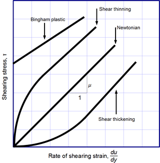
A fluid that behaves according to Newton's law, with a viscosity $μ$ that is independent of the stress, is said to be Newtonian. Gases, water, and many common liquids can be considered Newtonian in ordinary conditions and contexts. There are many non-Newtonian fluids that significantly deviate from that law in some way or other. For example:

Shear-thickening liquids, whose viscosity increases with the rate of shear strain.
Shear-thinning liquids, whose viscosity decreases with the rate of shear strain.
Thixotropic liquids, that become less viscous over time when shaken, agitated, or otherwise stressed.
Rheopectic (dilatant) liquids, that become more viscous over time when shaken, agitated, or otherwise stressed.
Bingham plastics that behave as a solid at low stresses but flow as a viscous fluid at high stresses.

Shear-thinning liquids are very commonly, but misleadingly, described as thixotropic.

Even for a Newtonian fluid, the viscosity usually depends on its composition and temperature. For gases and other compressible fluids, it depends on temperature and varies very slowly with pressure.

The viscosity of some fluids may depend on other factors. A magnetorheological fluid, for example, becomes thicker when subjected to a magnetic field, possibly to the point of behaving like a solid.

In solids

The viscous forces that arise during fluid flow must not be confused with the elastic forces that arise in a solid in response to shear, compression or extension stresses. While in the latter the stress is proportional to the amount of shear deformation, in a fluid it is proportional to the rate of deformation over time. (For this reason, Maxwell used the term fugitive elasticity for fluid viscosity.)

However, many liquids (including water) will briefly react like elastic solids when subjected to sudden stress. Conversely, many "solids" (even granite) will flow like liquids, albeit very slowly, even under arbitrarily small stress.^[11] Such materials are therefore best described as possessing both elasticity (reaction to deformation) and viscosity (reaction to rate of deformation); that is, being viscoelastic.

Indeed, some authors have claimed that amorphous solids, such as glass and many polymers, are actually liquids with a very high viscosity (greater than 10¹² Pa·s). ^[12] However, other authors dispute this hypothesis, claiming instead that there is some threshold for the stress, below which most solids will not flow at all,^[13] and that alleged instances of glass flow in window panes of old buildings are due to the crude manufacturing process of older eras rather than to the viscosity of glass.^[14]

Viscoelastic solids may exhibit both shear viscosity and bulk viscosity. The extensional viscosity is a linear combination of the shear and bulk viscosities that describes the reaction of a solid elastic material to elongation. It is widely used for characterizing polymers.

In geology, earth materials that exhibit viscous deformation at least three orders of magnitude greater than their elastic deformation are sometimes called rheids.^[15]

Measurement

Viscosity is measured with various types of viscometers and rheometers. A rheometer is used for those fluids that cannot be defined by a single value of viscosity and therefore require more parameters to be set and measured than is the case for a viscometer. Close temperature control of the fluid is essential to acquire accurate measurements, particularly in materials like lubricants, whose viscosity can double with a change of only 5 °C.

For some fluids, the viscosity is constant over a wide range of shear rates (Newtonian fluids). The fluids without a constant viscosity (non-Newtonian fluids) cannot be described by a single number. Non-Newtonian fluids exhibit a variety of different correlations between shear stress and shear rate.

One of the most common instruments for measuring kinematic viscosity is the glass capillary viscometer.

In coating industries, viscosity may be measured with a cup in which the efflux time is measured. There are several sorts of cup – such as the Zahn cup and the Ford viscosity cup – with the usage of each type varying mainly according to the industry. The efflux time can also be converted to kinematic viscosities (centistokes, cSt) through the conversion equations.^[16]

Also used in coatings, a Stormer viscometer uses load-based rotation in order to determine viscosity. The viscosity is reported in Krebs units (KU), which are unique to Stormer viscometers.

Vibrating viscometers can also be used to measure viscosity. Resonant, or vibrational viscometers work by creating shear waves within the liquid. In this method, the sensor is submerged in the fluid and is made to resonate at a specific frequency. As the surface of the sensor shears through the liquid, energy is lost due to its viscosity. This dissipated energy is then measured and converted into a viscosity reading. A higher viscosity causes a greater loss of energy.

Extensional viscosity can be measured with various rheometers that apply extensional stress.

Volume viscosity can be measured with an acoustic rheometer.

Apparent viscosity is a calculation derived from tests performed on drilling fluid used in oil or gas well development. These calculations and tests help engineers develop and maintain the properties of the drilling fluid to the specifications required.

Units

Dynamic viscosity, $μ$

The SI unit of dynamic viscosity is Pa·s or kg·m−1·s−1.

Both the physical unit of dynamic viscosity in SI units, the poiseuille (Pl), and cgs units, the poise (P), are named after Jean Léonard Marie Poiseuille. The poiseuille, which is rarely used, is equivalent to the pascal second (Pa·s), or (N·s)/m², or kg/(m·s). If a fluid is placed between two plates with distance one meter, and one plate is pushed sideways with a shear stress of one pascal, and it moves at $x$ meters per second, then it has viscosity of $1 / x$ pascal seconds. For example, water at 20 °C has a viscosity of 1.002 mPa·s, while a typical motor oil could have a viscosity of about 250 mPa·s.^[17] The units used in practice are either Pa·s and its submultiples or the cgs poise referred to below, and its submultiples.

The cgs physical unit for dynamic viscosity, the poise^[18] (P), is also named after Jean Poiseuille. It is more commonly expressed, particularly in ASTM standards, as centipoise (cP) since the latter is equal to the SI multiple millipascal seconds (mPa·s). For example, water at 20 °C has a viscosity of 1.002 mPa·s = 1.002 cP.

1 Pl = 1 Pa·s

1 P = 1 dPa·s = 0.1 Pa·s = 0.1 kg·m⁻¹·s⁻¹

1 cP = 1 mPa·s = 0.001 Pa·s = 0.001 N·s·m⁻² = 0.001 kg·m⁻¹·s⁻¹.

Kinematic viscosity, $ν$

The SI unit of kinematic viscosity is m²/s.

The cgs physical unit for kinematic viscosity is the stokes (St), named after Sir George Gabriel Stokes.^[19] It is sometimes expressed in terms of centistokes (cSt). In U.S. usage, stoke is sometimes used as the singular form.

1 St = 1 cm²·s⁻¹ = 10⁻⁴ m²·s⁻¹.

1 cSt = 1 mm²·s⁻¹ = 10⁻⁶m²·s⁻¹.

Water at 20 °C has a kinematic viscosity of about 10⁻⁶m²·s⁻¹ or 1 cSt.

The kinematic viscosity is sometimes referred to as diffusivity of momentum, because it is analogous to diffusivity of heat and diffusivity of mass. It is therefore used in dimensionless numbers which compare the ratio of the diffusivities.

Fluidity

The reciprocal of viscosity is fluidity, usually symbolized by $φ = 1 / μ$ or $F = 1 / μ$ , depending on the convention used, measured in reciprocal poise (P⁻¹, or cm·s·g⁻¹), sometimes called the rhe. Fluidity is seldom used in engineering practice.

The concept of fluidity can be used to determine the viscosity of an ideal solution. For two components A and B, the fluidity when A and B are mixed is

F\approx \chi _{\mathrm {A} }F_{\mathrm {A} }+\chi _{\mathrm {B} }F_{\mathrm {B} },

which is only slightly simpler than the equivalent equation in terms of viscosity:

\mu \approx {\frac {1}{{\dfrac {\chi _{\mathrm {A} }}{\mu _{\mathrm {A} }}}+{\dfrac {\chi _{\mathrm {B} }}{\mu _{\mathrm {B} }}}}},

where $χ A$ and $χ B$ are the mole fractions of components A and B respectively, and $μ A$ and $μ B$ are the components' pure viscosities.

Non-standard units

The reyn is a British unit of dynamic viscosity.

Viscosity index is a measure for the change of viscosity with temperature. It is used in the automotive industry to characterise lubricating oil.

At one time the petroleum industry relied on measuring kinematic viscosity by means of the Saybolt viscometer, and expressing kinematic viscosity in units of Saybolt universal seconds (SUS).^[20] Other abbreviations such as SSU (Saybolt seconds universal) or SUV (Saybolt universal viscosity) are sometimes used. Kinematic viscosity in centistokes can be converted from SUS according to the arithmetic and the reference table provided in ASTM D 2161.^[21]

Molecular origins

Pitch has a viscosity approximately 230 billion (2.3×10¹¹) times that of water.^[22]

In general, the viscosity of a system depends in detail on how the molecules constituting the system interact. There are no simple but correct expressions for the viscosity of a fluid. The simplest exact expressions are the Green–Kubo relations for the linear shear viscosity or the transient time correlation function expressions derived by Evans and Morriss in 1985.^[23] Although these expressions are each exact, calculating the viscosity of a dense fluid using these relations currently requires the use of molecular dynamics computer simulations. On the other hand, much more progress can be made for a dilute gas. Even elementary assumptions about how gas molecules move and interact lead to a basic understanding of the molecular origins of viscosity. More sophisticated treatments can be constructed by systematically coarse-graining the equations of motion of the gas molecules. An example of such a treatment is Chapman–Enskog theory, which derives expressions for the viscosity of a dilute gas from the Boltzmann equation.^[24]

Momentum transport in gases is generally mediated by discrete molecular collisions, and in liquids by attractive forces which bind molecules close together.^[25] Because of this, the dynamic viscosities of liquids are typically several orders of magnitude higher than dynamic viscosities of gases.

Gases

Viscosity in gases arises principally from the molecular diffusion that transports momentum between layers of flow. An elementary calculation for a dilute gas at temperature $T$ and density $\rho$ gives

\mu =\alpha \rho \lambda {\sqrt {\frac {2k_{B}T}{\pi m}}},

where $k_{B}$ is the Boltzmann constant, $m$ the molecular mass, and $\alpha$ a numerical constant on the order of $1$ . The quantity $\lambda$ , the mean free path, measures the average distance a molecule travels between collisions. Even without a priori knowledge of $\alpha$ , this expression has interesting implications. In particular, since $\lambda$ is typically inversely proportional to density and increases with temperature, $\mu$ itself should increase with temperature and be independent of density. In fact, both of these predictions persist in more sophisticated treatments, and accurately describe experimental observations. Note that this behavior runs counter to common intuition regarding liquids, for which viscosity typically decreases with temperature.^[25]^[26]

Elementary calculation of viscosity for a dilute gas^[27]

Consider a dilute gas moving parallel to the $x$ -axis with velocity $u(y)$ that depends only on the $y$ coordinate. To simplify the discussion, the gas is assumed to have uniform temperature and density.

Under these assumptions, the $x$ velocity of a molecule passing through $y=0$ is equal to whatever velocity that molecule had when its mean free path $\lambda$ began. Because $\lambda$ is typically small compared with macroscopic scales, the average $x$ velocity of such a molecule has the form

u(0)\pm \alpha \lambda {\frac {du}{dy}}(0)

,

where $\alpha$ is a numerical constant on the order of $1$ . (Some authors estimate $\alpha =2/3$ ;^[25]^[26] on the other hand, a more careful calculation for rigid elastic spheres gives $\alpha \simeq 0.998$ .) Now, because half the molecules on either side are moving towards $y=0$ , and doing so on average with half the average moleculer speed $(8k_{B}T/\pi m)^{1/2}$ , the momentum flux from either side is

{\frac {1}{4}}\rho \cdot {\sqrt {\frac {8k_{B}T}{\pi m}}}\cdot \left(u(0)\pm \alpha \lambda {\frac {du}{dy}}(0)\right).

The net momentum flux at $y=0$ is the difference of the two:

-{\frac {1}{2}}\rho \cdot {\sqrt {\frac {8k_{B}T}{\pi m}}}\cdot \alpha \lambda {\frac {du}{dy}}(0).

According to the definition of viscosity, this momentum flux should be equal to $-\mu {\frac {du}{dy}}(0)$ , which leads to

\mu =\alpha \rho \lambda {\sqrt {\frac {2k_{B}T}{\pi m}}}.

For rigid elastic spheres of diameter $\sigma$ , $\lambda$ can be computed, giving

\mu ={\frac {\alpha }{\pi ^{3/2}}}{\frac {\sqrt {k_{B}mT}}{\sigma ^{2}}}.

In this case $\lambda$ is independent of temperature, so $\mu \propto T^{1/2}$ . For more complicated molecular models, however, $\lambda$ depends on temperature in a non-trivial way, and simple kinetic arguments as used here are inadequate. More fundamentally, the notion of a mean free path becomes imprecise for particles that interact over a finite range, which limits the usefulness of the concept for describing real-world gases.^[28]

Chapman–Enskog theory

A technique developed by Sydney Chapman and David Enskog in the early 1900s allows a more refined calculation of $\mu$ .^[24] It is based on the Boltzmann equation, which provides a systematic statistical description of a dilute gas in terms of intermolecular interactions.^[29] As such, their technique allows accurate calculation of $\mu$ for more realistic molecular models, such as those incorporating intermolecular attraction rather than just hard-core repulsion.

It turns out that a more realistic modeling of interactions is essential for accurate prediction of the temperature dependence of $\mu$ , which experiments show increases more rapidly than the $T^{1/2}$ trend predicted for rigid elastic spheres.^[25] Indeed, the Chapman–Enskog analysis shows that the predicted temperature dependence can be tuned by varying the parameters in various molecular models. A simple example is the Sutherland model,^[30] which describes rigid elastic spheres with weak mutual attraction. In such a case, the attractive force can be treated perturbatively, which leads to a particularly simple expression for $\mu$ :

\mu ={\frac {5}{16\sigma ^{2}}}\left({\frac {k_{B}mT}{\pi }}\right)^{1/2}\left(1+{\frac {S}{T}}\right)^{-1},

where $S$ is independent of temperature, being determined only by the parameters of the intermolecular attraction. To connect with experiment, it is convenient to rewrite as

\mu =\mu _{0}\left({\frac {T}{T_{0}}}\right)^{3/2}{\frac {T_{0}+S}{T+S}},

where $\mu _{0}$ is the viscosity at temperature $T_{0}$ . If $\mu$ is known from experiments at $T=T_{0}$ and at least one other temperature, then $S$ can be calculated. It turns out that expressions for $\mu$ obtained in this way are accurate for a number of gases over a sizable range of temperatures. On the other hand, Chapman and Cowling^[24] argue that this success does not imply that molecules actually interact according to the Sutherland model. Rather, they interpret the prediction for $\mu$ as a simple interpolation which is valid for some gases over fixed ranges of temperature, but otherwise does not provide a picture of intermolecular interactions which is fundamentally correct and general. Slightly more sophisticated models, such as the Lennard–Jones potential, may provide a better picture, but only at the cost of a more opaque dependence on temperature. In some systems the assumption of spherical symmetry must be abandoned as well, as is the case for vapors with highly polar molecules like H₂O.^[31]^[32]

Liquids

In contrast with gases, there is no simple yet accurate picture for the molecular origins of viscosity in liquids.

At the simplest level of description, the relative motion of adjacent layers in a liquid is opposed primarily by attractive molecular forces acting across the layer boundary. In this picture, one (correctly) expects viscosity to decrease with temperature. This is because increasing temperature increases the random thermal motion of the molecules, which makes it easier for them to overcome their attractive interactions.^[33]

Building on this visualization, a simple theory can be constructed in analogy with the discrete structure of a solid: groups of molecules in a liquid are visualized as forming "cages" which surround and enclose single molecules.^[34] These cages can be occupied or unoccupied, and stronger molecular attraction corresponds to stronger cages. Due to random thermal motion, a molecule "hops" between cages at a rate which varies inversely with the strength of molecular attractions. In equilibrium these "hops" are not biased in any direction. On the other hand, in order for two adjacent layers to move relative to each other, the "hops" must be biased in the direction of the relative motion. The force required to sustain this directed motion can be estimated for a given shear rate, leading to

$\mu \approx {\frac {N_{A}h}{V}}{\text{exp}}(3.8T_{b}/T),$

(1)

where $N_{A}$ is the Avogadro constant, $h$ is the Planck constant, $V$ is the volume of a mole of liquid, and $T_{b}$ is the normal boiling point. This result has the same form as the widespread and accurate empirical relation

$\mu =Ae^{B/T},$

(2)

where $A$ and $B$ are constants fit from data.^[34]^[35] One the other hand, several authors express caution with respect to this model. Errors as large as 30% can be encountered using equation (1), compared with fitting equation (2) to experimental data.^[34] More fundamentally, the physical assumptions underlying equation (1) have been extensively criticized.^[36] It has also been argued that the exponential dependence in equation (1) does not necessarily describe experimental observations more accurately than simpler, non-exponential expressions.^[37]^[38]

In light of these shortcomings, the development of a less ad-hoc model is a matter of practical interest. Foregoing simplicity in favor of precision, it is possible to write rigorous expressions for viscosity starting from the fundamental equations of motion for molecules. A classic example of this approach is Irving-Kirkwood theory.^[39] On the other hand, such expressions are given as averages over multiparticle correlation functions and are therefore difficult to apply in practice.

In general, empirically derived expressions (based on existing viscosity measurements) appear to be the only consistently reliable means of calculating viscosity in liquids.^[40]

Selected substances

Air

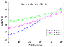
Pressure dependence of the dynamic viscosity of dry air at the temperatures of 300, 400 and 500 kelvins

The viscosity of air depends mostly on the temperature. At 15 °C, the viscosity of air is 6995181000000000000♠1.81×10⁻⁵ kg/(m·s), 18.1 μPa·s or 6995181000000000000♠1.81×10⁻⁵ Pa·s. The kinematic viscosity at 15 °C is 6995148000000000000♠1.48×10⁻⁵ m²/s or 14.8 cSt. At 25 °C, the viscosity is 18.6 μPa·s and the kinematic viscosity 15.7 cSt.

Water

Dynamic viscosity of water

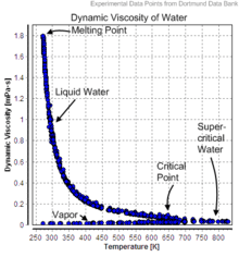
The dynamic viscosity of water is 6996890000000000000♠8.90×10⁻⁴ Pa·s or 6997890000000000000♠8.90×10⁻³ dyn·s/cm² or 0.890 cP at about 25 °C.

As a function of temperature $T$ (in kelvins): $μ = A \times 10 B /(T - C)$ , where $A$ = 6995241400000000000♠2.414×10⁻⁵ Pa·s, $B$ = 247.8 K, and $C$ = 140 K.

The dynamic viscosity of liquid water at different temperatures up to the normal boiling point is listed below.

Dynamic viscosity of water at various temperatures
Temperature (°C)	Viscosity (mPa·s)
10	1.308
20	1.002
30	0.7978
40	0.6531
50	0.5471
60	0.4658
70	0.4044
80	0.3550
90	0.3150
100	0.2822

Other substances

Example of the viscosity of milk and water. Liquids with higher viscosities make smaller splashes when poured at the same velocity.

Honey being drizzled

Peanut butter is a semi-solid and can therefore hold peaks.

Some dynamic viscosities of Newtonian fluids are listed below:

Viscosity of selected gases at 100 kPa (μPa·s)
Gas	at 0 °C (273 K)	at 27 °C (300 K)^[41]
air	17.4	18.6
hydrogen	8.4	9.0
helium		20.0
argon		22.9
xenon	21.2	23.2
carbon dioxide		15.0
methane		11.2
ethane		9.5

Viscosity of fluids with variable compositions
Fluid	Viscosity (Pa·s)	Viscosity (cP)
blood (37 °C)^[12]	6997300000000000000♠3×10⁻³ – 6997400000000000000♠4×10⁻³	3–4
honey	2–10^[42]	2000–7004100000000000000♠10000
molasses	5–10	5000–7004100000000000000♠10000
molten glass	10–1000	7004100000000000000♠10000–7006100000000000000♠1000000
chocolate syrup	10–25	7004100000000000000♠10000–7004250000000000000♠25000
molten chocolate^{[lower-alpha 1]}	45–130^[43]	7004450000000000000♠45000–7005130000000000000♠130000
ketchup^{[lower-alpha 1]}	50–100	7004500000000000000♠50000–7005100000000000000♠100000
lard	≈ 100	≈ 7005100000000000000♠100000
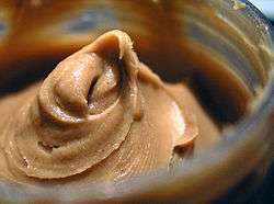
peanut butter^{[lower-alpha 1]}	≈ 250	≈ 7005250000000000000♠250000
shortening^{[lower-alpha 1]}	≈ 250	≈ 7005250000000000000♠250000

Viscosity of liquids
(at 25 °C unless otherwise specified)
Liquid	Viscosity (Pa·s)	Viscosity (cP)
acetone^[41]	6996306000000000000♠3.06×10⁻⁴	0.306
benzene^[41]	6996604000000000000♠6.04×10⁻⁴	0.604
castor oil^[41]	0.985	985
corn syrup^[41]	1.3806	1380.6
ethanol^[41]	6997107400000000000♠1.074×10⁻³	7000107400000000000♠1.074
ethylene glycol	6998161000000000000♠1.61×10⁻²	7001161000000000000♠16.1
glycerol (at 20 °C)^[44]	7000120000000000000♠1.2	7003120000000000000♠1200
HFO-380	7000202199999999999♠2.022	7003202200000000000♠2022
mercury^[41]	6997152600000000000♠1.526×10⁻³	7000152600000000000♠1.526
methanol^[41]	6996544000000000000♠5.44×10⁻⁴	6999544000000000000♠0.544
motor oil SAE 10 (20 °C)^[45]	6998650000000000000♠0.065	7001650000000000000♠65
motor oil SAE 40 (20 °C)^[45]	6999319000000000000♠0.319	7002319000000000000♠319
nitrobenzene^[41]	6997186300000000000♠1.863×10⁻³	7000186300000000000♠1.863
liquid nitrogen (−196 °C)	6996158000000000000♠1.58×10⁻⁴	6999158000000000000♠0.158
propanol^[41]	6997194500000000000♠1.945×10⁻³	7000194500000000000♠1.945
olive oil	6998810000000000000♠0.081	7001810000000000000♠81
pitch	7008229999999999999♠2.3×10⁸	7011229999999999999♠2.30×10¹¹
sulfuric acid^[41]	6998242000000000000♠2.42×10⁻²	7001242000000000000♠24.2
water	6996894000000000000♠8.94×10⁻⁴	6999894000000000000♠0.894

Viscosity of solids
Solid	Viscosity (Pa·s)	Temperature (°C)
granite^[11]	7019300000000000000♠3×10¹⁹ - 7019600000000000000♠6×10¹⁹	25
asthenosphere^[46]	7019700000000000000♠7.0×10¹⁹	900
upper mantle^[46]	7020700000000000000♠7×10²⁰ – 7021100000000000000♠1×10²¹	1300–3000
lower mantle	7021100000000000000♠1×10²¹ – 7021200000000000000♠2×10²¹	3000–4000

1 2 3 4 These materials are highly non-Newtonian.

Blends of liquids

The viscosity of the blend of two or more liquids can be estimated using the Refutas equation.^[47]^[48] The calculation is carried out in three steps.

The first step is to calculate the viscosity blending number (VBN) (also called the viscosity blending index) of each component of the blend:

\mathrm {VBN} =14.534\times \ln {\big (}\ln(\nu +0.8){\big )}+10.975\,

(1)

where $ν$ is the kinematic viscosity in centistokes (cSt). It is important that the kinematic viscosity of each component of the blend be obtained at the same temperature.

The next step is to calculate the VBN of the blend, using this equation:

\mathrm {VBN_{Blend}} =\left(x_{\mathrm {A} }\times \mathrm {VBN_{A}} \right)+\left(x_{\mathrm {B} }\times \mathrm {VBN_{B}} \right)+\cdots +\left(x_{\mathrm {N} }\times \mathrm {VBN_{N}} \right)\,

(2)

where $x X$ is the mass fraction of each component of the blend.

Once the viscosity blending number of a blend has been calculated using equation (2), the final step is to determine the kinematic viscosity of the blend by solving equation (1) for $ν$ :

\nu =\exp \left(\exp \left({\frac {\mathrm {VBN_{Blend}} -10.975}{14.534}}\right)\right)-0.8,

(3)

where $VBN Blend$ is the viscosity blending number of the blend.

alternatively use the more accurate Lederer-Roegiers equation

$\ln \eta _{1,2}={\frac {x_{1}\ln \eta _{1}}{x_{1}+x_{2}\beta }}+{\frac {\beta x_{2}\ln \eta _{2}}{x_{1}+x_{2}\beta }}$

$\beta$ is based on the difference in intermolecular cohesion energies between the liquids
$\eta$ =dynamic viscosity
$x_{i}$ =mole fraction of particle species $i$

Slurry

Plot of slurry relative viscosity

μ r

as calculated by empirical correlations from Einstein,^[49] Guth and Simha,^[50] Thomas,^[51] and Kitano et al.^[52]

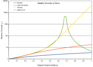
The term slurry describes mixtures of a liquid and solid particles that retain some fluidity. The viscosity of slurry can be described as relative to the viscosity of the liquid phase:

\mu _{\mathrm {s} }=\mu _{\mathrm {r} }\mu _{\mathrm {l} },

where $μ s$ and $μ l$ are respectively the dynamic viscosity of the slurry and liquid (Pa·s), and $μ r$ is the relative viscosity (dimensionless).

Depending on the size and concentration of the solid particles, several models exist that describe the relative viscosity as a function of volume fraction $φ$ of solid particles.

In the case of extremely low concentrations of fine particles, Einstein's equation^[49] may be used:

\mu _{\mathrm {r} }=1+2.5\varphi

In the case of higher concentrations, a modified equation was proposed by Guth and Simha,^[50] which takes into account interaction between the solid particles:

\mu _{\mathrm {r} }=1+2.5\varphi +14.1\varphi ^{2}

Further modification of this equation was proposed by Thomas^[51] from the fitting of empirical data:

\mu _{\mathrm {r} }=1+2.5\varphi +10.05\varphi ^{2}+Ae^{B\varphi },

where $A$ = 6997272999999999999♠0.00273 and $B$ = 16.6.

In the case of high shear stress (above 1 kPa), another empirical equation was proposed by Kitano et al. for polymer melts:^[52]

\mu _{\mathrm {r} }=\left(1-{\frac {\varphi }{A}}\right)^{-2},

where $A$ = 0.68 for smooth spherical particles.

Nanofluids

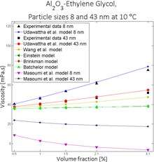
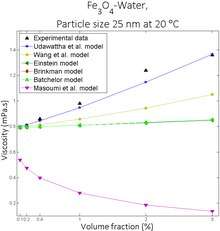
Alumina-ethylene glycol, particle sizes 8 and 43 nm at 10 Celsius

Magnatite-water, particle sizes 25nm at 20 Celsius

Nanofluid is a novel class of fluid, which is developed by dispersing nano-sized particles in base fluid.^[53]

Einstein model

Einstein derived the applicable first theoretical formula for the estimation of viscosity values of composites or mixtures in 1906. This model developed while assuming linear viscous fluid including suspensions of rigid and spherical particles. Einstein’s model is valid for very low volume fraction $\varnothing$ .^[49]

$\mu _{nf}=\mu _{bf}(1+2.5\varnothing )$

Brinkman model

Brinkman modified Einstein’s model for used with average particle volume fraction up to 4%^[54]

$\mu _{nf}=\mu _{bf}{\Biggl (}{\frac {1}{\ (1-\varnothing )^{2.5}}}{\Biggr )}=\mu _{bf}{\Big (}1+2.5\varnothing +4.375\varnothing ^{2}+O(\varnothing ^{3}){\Big )}$

Batchelor model

Batchelor reformed Einstein's theoretical model by presenting Brownian motion effect.^[55]

$\mu _{nf}=\mu _{bf}(1+2.5\varnothing +6.5{\varnothing }^{2})$

Wang et al. model

Wang et al. found a model to predict viscosity of nanofluid as follows.^[56]

$\mu _{nf}=\mu _{bf}(1+7.3\varnothing +123{\varnothing }^{2})$

Masoumi et al. model

Masoumi et al. suggested a new viscosity correlation by considering Brownian motion of nanoparticle in nanofluid.^[57]

$\mu _{nf}=\mu _{bf}{\Biggl (}1+{\frac {\rho _{p}V_{B}{d_{p}}^{2}}{72\delta C}}{\Biggr )}$

$V_{B}={\sqrt {\frac {18K_{B}T}{\pi \rho _{p}{d_{p}}^{3}}}}$

$\delta ={\sqrt[{3}]{\frac {\pi {d_{p}}^{3}}{6\varnothing }}}$

$C=\{{(-1.133d_{p}-2.771)\varnothing +(0.09d_{p}-0.393)}\}\times 10^{-6}$

Udawattha et al. model

Udawattha et al. modified the Masoumi et al. model. The developed model valid for suspension containing micro-size particles.^[58]

$\mu _{nf}=\mu _{bf}{\Biggl (}1+2.5\varnothing _{e}+{\frac {\rho _{p}V_{B}{d_{p}}^{2}}{72\delta [T\times 10^{-10}\times \varnothing ^{-0.002T-0.284}]}}{\Biggr )}$

$\varnothing _{e}=\varnothing {{\Biggl (}1+{\frac {h}{r}}{\Biggr )}}^{3}$

where

\mu

is the viscosity of the sample, in [Pa·s]

nf

is nanofluid

bf

is basefluid

p

is particle

\varnothing

is volume fraction

\rho

is density of the sample, in [kg·m⁻³]

\delta

is distance between two particles

V_{B}

is Brownian motion of particle

K_{B}

is the Boltzmann constant

T

is Temperature of the sample, in [K]

d_{p}

is diameter of a particle

h

is nanolayer thickness (1 nm)

r

is radius of a particle

Amorphous materials

Common glass viscosity curves^[59]

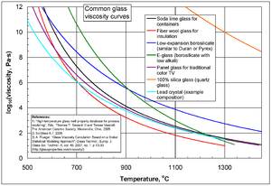
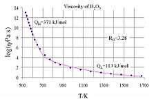
Viscous flow in amorphous materials (e.g. in glasses and melts)^[60]^[61]^[62] is a thermally activated process:

\mu =Ae^{\frac {Q}{RT}},

where $Q$ is activation energy, $T$ is temperature, $R$ is the molar gas constant and $A$ is approximately a constant.

The viscous flow in amorphous materials is characterized by a deviation from the Arrhenius-type behavior: $Q$ changes from a high value $Q H$ at low temperatures (in the glassy state) to a low value $Q L$ at high temperatures (in the liquid state). Depending on this change, amorphous materials are classified as either

strong when: $Q H - Q L < Q L$ or
fragile when: $Q H - Q L \geq Q L$ .

The fragility of amorphous materials is numerically characterized by Doremus' fragility ratio:

R_{\mathrm {D} }={\frac {Q_{\mathrm {H} }}{Q_{\mathrm {L} }}}

and strong materials have $R D < 2$ whereas fragile materials have $R D \geq 2$ .

Common logarithm of viscosity against temperature for B₂O₃, showing two regimes

The viscosity of amorphous materials is quite exactly described by a two-exponential equation:

\mu =A_{1}T\left(1+A_{2}e^{\frac {B}{RT}}\right)\left(1+Ce^{\frac {D}{RT}}\right),

with constants $A 1$ , $A 2$ , $B$ , $C$ and $D$ related to thermodynamic parameters of joining bonds of an amorphous material.

Not very far from the glass transition temperature, $T g$ , this equation can be approximated by a Vogel–Fulcher–Tammann (VFT) equation.

If the temperature is significantly lower than the glass transition temperature, $T ≪ T g$ , then the two-exponential equation simplifies to an Arrhenius-type equation:

\mu =A_{\mathrm {L} }Te^{\frac {Q_{\mathrm {H} }}{RT}}

with

Q_{\mathrm {H} }=H_{\mathrm {d} }+H_{\mathrm {m} },

where $H d$ is the enthalpy of formation of broken bonds (termed configurons^[63]) and $H m$ is the enthalpy of their motion.

When the temperature is less than the glass transition temperature, $T < T g$ , the activation energy of viscosity is high because the amorphous materials are in the glassy state and most of their joining bonds are intact.

If the temperature is much higher than the glass transition temperature, $T ≫ T g$ , the two-exponential equation also simplifies to an Arrhenius-type equation:

\mu =A_{\mathrm {H} }Te^{\frac {Q_{\mathrm {L} }}{RT}},

with

Q_{\mathrm {L} }=H_{\mathrm {m} }.

When the temperature is higher than the glass transition temperature, $T > T g$ , the activation energy of viscosity is low because amorphous materials are melted and have most of their joining bonds broken, which facilitates flow.

Eddy viscosity

In the study of turbulence in fluids, a common practical strategy for calculation is to ignore the small-scale vortices (or eddies) in the motion and to calculate a large-scale motion with an eddy viscosity that characterizes the transport and dissipation of energy in the smaller-scale flow (see large eddy simulation). Values of eddy viscosity used in modeling ocean circulation may be from 7004500000000000000♠5×10⁴ to 7006100000000000000♠1×10⁶ Pa·s depending upon the resolution of the numerical grid.

References

↑ "viscosity". Merriam-Webster Dictionary.
↑ Symon, Keith (1971). Mechanics (3rd ed.). Addison-Wesley. ISBN 978-0-201-07392-8.
↑ "viscous". Etymonline.com. Retrieved 2010-09-14.
↑ Streeter, Victor Lyle; Wylie, E. Benjamin; Bedford, Keith W. (1998). Fluid Mechanics. McGraw-Hill. ISBN 978-0-07-062537-2.
↑ Holman, J. P. (2002). Heat Transfer. McGraw-Hill. ISBN 978-0-07-122621-9.
↑ Incropera, Frank P.; DeWitt, David P. (2007). Fundamentals of Heat and Mass Transfer. Wiley. ISBN 978-0-471-45728-2.
↑ Nič, Miloslav; Jirát, Jiří; Košata, Bedřich; Jenkins, Aubrey, eds. (1997). "dynamic viscosity, η". IUPAC Compendium of Chemical Terminology. Oxford: Blackwell Scientific Publications. doi:10.1351/goldbook. ISBN 978-0-9678550-9-7.
↑ Bird, R. Byron; Stewart, Warren E.; Lightfoot, Edwin N. (2007), Transport Phenomena (2nd ed.), John Wiley & Sons, Inc., p. 19, ISBN 978-0-470-11539-8
↑ Bird, Steward, & Lightfoot, p. 18 (Note that this source uses a alternate sign convention, which has been reversed here.)
1 2 Bird, Steward, & Lightfoot, p. 19
1 2 Kumagai, Naoichi; Sasajima, Sadao; Ito, Hidebumi (15 February 1978). "Long-term Creep of Rocks: Results with Large Specimens Obtained in about 20 Years and Those with Small Specimens in about 3 Years". Journal of the Society of Materials Science (Japan). 27 (293): 157–161. Retrieved 2008-06-16.
1 2 Elert, Glenn. "Viscosity". The Physics Hypertextbook.
↑ Gibbs, Philip. "Is Glass a Liquid or a Solid?". Retrieved 2007-07-31.
↑ Plumb, Robert C. (1989). "Antique windowpanes and the flow of supercooled liquids". Journal of Chemical Education. 66 (12): 994. Bibcode:1989JChEd..66..994P. doi:10.1021/ed066p994.
↑ Scherer, George W.; Pardenek, Sandra A.; Swiatek, Rose M. (1988). "Viscoelasticity in silica gel". Journal of Non-Crystalline Solids. 107 (1): 14. Bibcode:1988JNCS..107...14S. doi:10.1016/0022-3093(88)90086-5.
↑ "Viscosity" (PDF). BYK-Gardner.
↑ Serway, Raymond A. (1996). Physics for Scientists & Engineers (4th ed.). Saunders College Publishing. ISBN 978-0-03-005932-2.
↑ "IUPAC definition of the Poise". Retrieved 2010-09-14.
↑ Gyllenbok, Jan (2018). "Encyclopaedia of Historical Metrology, Weights, and Measures". Encyclopaedia of Historical Metrology, Weights, and Measures, Volume 1. Birkhäuser. p. 213. ISBN 9783319575988.
↑ ASTM D 2161 (2005) "Standard Practice for Conversion of Kinematic Viscosity to Saybolt Universal Viscosity or to Saybolt Furol Viscosity", p. 1
↑ "Quantities and Units of Viscosity". Uniteasy.com. Retrieved 2010-09-14.
↑ Edgeworth, R.; Dalton, B. J.; Parnell, T. (1984). "The pitch drop experiment". European Journal of Physics. 5 (4): 198–200. Bibcode:1984EJPh....5..198E. doi:10.1088/0143-0807/5/4/003. Retrieved 2009-03-31.
↑ Evans, Denis J.; Morriss, Gary P. (October 15, 1988). "Transient-time-correlation functions and the rheology of fluids". Physical Review A. 38 (8): 4142–4148. Bibcode:1988PhRvA..38.4142E. doi:10.1103/PhysRevA.38.4142. PMID 9900865.
1 2 3 Chapman, Sydney; Cowling, T.G. (1970), The Mathematical Theory of Non-Uniform Gases (3rd ed.), Cambridge University Press
1 2 3 4 Bird, R. Byron; Stewart, Warren E.; Lightfoot, Edwin N. (2007), Transport Phenomena (2nd ed.), John Wiley & Sons, Inc., ISBN 978-0-470-11539-8
1 2 Bellac, Michael; Mortessagne, Fabrice; Batrouni, G. George (2004), Equilibrium and Non-Equilibrium Statistical Thermodynamics, Cambridge University Press, ISBN 978-0-521-82143-8
↑ Chapman & Cowling, pp. 97-98
↑ Chapman & Cowling, p. 103
↑ Cercignani, Carlo (1975), Theory and Application of the Boltzmann Equation, Elsevier, ISBN 978-0-444-19450-3
↑ The discussion which follows draws from Chapman & Cowling, pp. 232-237.
↑ Bird, Steward, & Lightfoot, p. 25-27
↑ Chapman & Cowling, pp. 235 - 237
↑ Reid, Robert C.; Sherwood, Thomas K. (1958), The Properties of Gases and Liquids, McGraw-Hill Book Company, Inc., p. 202
1 2 3 Bird, Steward, & Lightfoot, pp. 29-31
↑ Reid & Sherwood, pp. 203-204
↑ Hildebrand, Joel Henry (1977), Viscosity and Diffusivity: A Predictive Treatment, John Wiley & Sons, Inc., ISBN 0-471-03072-4
↑ Hildebrand p. 37
↑ Egelstaff, P.A. (1992), An Introduction to the Liquid State (2nd ed.), Oxford University Press, p. 264, ISBN 0-19-851012-8
↑ Irving, J.H.; Kirkwood, John G. (1949), "The Statistical Mechanical Theory of Transport Processes. IV. The Equations of Hydrodynamics", J. Chem. Phys., 18 (6)
↑ Reid & Sherwood, pp. 206-209
1 2 3 4 5 6 7 8 9 10 11 Lide, D. R., ed. (2005). CRC Handbook of Chemistry and Physics (86th ed.). Boca Raton (FL): CRC Press. ISBN 0-8493-0486-5.
↑ Yanniotis, S.; Skaltsi, S.; Karaburnioti, S. (February 2006). "Effect of moisture content on the viscosity of honey at different temperatures". Journal of Food Engineering. 72 (4): 372–377. doi:10.1016/j.jfoodeng.2004.12.017.
↑ "Chocolate Processing". Brookfield Engineering website. Archived from the original on 2007-11-28. Retrieved 2007-12-03.
↑ "Viscosity of liquids and gases". GSU Hyperphysics.
1 2 Elert, Glenn. "The Physics Hypertextbook – Viscosity". Physics.info. Retrieved 2010-09-14.
1 2 Fjeldskaar, W. (1994). "Viscosity and thickness of the asthenosphere detected from the Fennoscandian uplift". Earth and Planetary Science Letters. 126 (4): 399–410. Bibcode:1994E&PSL.126..399F. doi:10.1016/0012-821X(94)90120-1.
↑ Maples, Robert E. (2000). Petroleum Refinery Process Economics (2nd ed.). Pennwell Books. ISBN 978-0-87814-779-3.
↑ "Lube-Tech - Viscosity Blending Equations" (PDF). Archived from the original (PDF) on 2016-05-27.
1 2 3 Einstein, A. (1906). "Eine neue Bestimmung der Moleküldimensionen". Annalen der Physik. 19 (2): 289–306. Bibcode:1906AnP...324..289E. doi:10.1002/andp.19063240204. hdl:20.500.11850/139872.
1 2 Guth, E.; Simha, R. (1936). "Untersuchungen über die Viskosität von Suspensionen und Lösungen. 3. Über die Viskosität von Kugelsuspensionen". Kolloid Z. 74 (3): 266. doi:10.1007/BF01428643.
1 2 Thomas, D. G. (1965). "Transport characteristics of suspension: VIII. A note on the viscosity of Newtonian suspensions of uniform spherical particles". J. Colloid Sci. 20 (3): 267–277. doi:10.1016/0095-8522(65)90016-4.
1 2 Kitano, T.; Kataoka, T.; Shirota, T. (1981). "An empirical equation of the relative viscosity of polymer melts filled with various inorganic fillers". Rheologica Acta. 20 (2): 207. doi:10.1007/BF01513064.
↑ Kasaeian, Alibakhsh; Eshghi, Amin Toghi; Sameti, Mohammad (2015-03-01). "A review on the applications of nanofluids in solar energy systems". Renewable and Sustainable Energy Reviews. 43 (Supplement C): 584–598. doi:10.1016/j.rser.2014.11.020.
↑ Brinkman, H. C. (1952-04-01). "The Viscosity of Concentrated Suspensions and Solutions". The Journal of Chemical Physics. 20 (4): 571. Bibcode:1952JChPh..20..571B. doi:10.1063/1.1700493. ISSN 0021-9606.
↑ Batchelor, G. K. (November 1977). "The effect of Brownian motion on the bulk stress in a suspension of spherical particles". Journal of Fluid Mechanics. 83 (1): 97–117. Bibcode:1977JFM....83...97B. doi:10.1017/S0022112077001062. ISSN 1469-7645.
↑ Wang, Xinwei; Xu, Xianfan; Choi, Stephen U. S. (1999). "Thermal Conductivity of Nanoparticle - Fluid Mixture". Journal of Thermophysics and Heat Transfer. 13 (4): 474–480. CiteSeerX 10.1.1.585.9136. doi:10.2514/2.6486. ISSN 0887-8722.
↑ Masoumi, N.; Sohrabi, N.; Behzadmehr, A. (2009). "A new model for calculating the effective viscosity of nanofluids". Journal of Physics D: Applied Physics. 42 (5): 055501. Bibcode:2009JPhD...42e5501M. doi:10.1088/0022-3727/42/5/055501. ISSN 0022-3727.
↑ Udawattha, Dilan S.; Narayana, Mahinsasa; Wijayarathne, Uditha P. L. (2017). "Predicting the effective viscosity of nanofluids based on the rheology of suspensions of solid particles". Journal of King Saud University - Science. doi:10.1016/j.jksus.2017.09.016.
↑ Fluegel, Alexander. "Viscosity calculation of glasses". Glassproperties.com. Retrieved 2010-09-14.
↑ Doremus, R. H. (2002). "Viscosity of silica". J. Appl. Phys. 92 (12): 7619–7629. Bibcode:2002JAP....92.7619D. doi:10.1063/1.1515132.
↑ Ojovan, M. I.; Lee, W. E. (2004). "Viscosity of network liquids within Doremus approach". J. Appl. Phys. 95 (7): 3803–3810. Bibcode:2004JAP....95.3803O. doi:10.1063/1.1647260.
↑ Ojovan, M. I.; Travis, K. P.; Hand, R. J. (2000). "Thermodynamic parameters of bonds in glassy materials from viscosity-temperature relationships". J. Phys.: Condens. Matter. 19 (41): 415107. Bibcode:2007JPCM...19O5107O. doi:10.1088/0953-8984/19/41/415107. PMID 28192319.
↑ "Configuron". Wikidoc.

External links

Fluid properties - high accuracy calculation of viscosity for frequently encountered pure liquids and gases
Gas viscosity calculator as function of temperature
Air viscosity calculator as function of temperature and pressure
Fluid Characteristics Chart - a table of viscosities and vapor pressures for various fluids
Gas Dynamics Toolbox - calculate coefficient of viscosity for mixtures of gases
Glass Viscosity Measurement - viscosity measurement, viscosity units and fixpoints, glass viscosity calculation
Kinematic Viscosity - conversion between kinematic and dynamic viscosity
Physical Characteristics of Water - a table of water viscosity as a function of temperature
Vogel–Tammann–Fulcher Equation Parameters
Calculation of temperature-dependent dynamic viscosities for some common components
"Test Procedures for Testing Highway and Nonroad Engines and Omnibus Technical Amendments" - United States Environmental Protection Agency
Artificial viscosity
Viscosity of Air, Dynamic and Kinematic, Engineers Edge

This article is issued from Wikipedia. The text is licensed under Creative Commons - Attribution - Sharealike. Additional terms may apply for the media files.

[nnf-43] 1 2 3 4 These materials are highly non-Newtonian.

[1] "viscosity". Merriam-Webster Dictionary.

[2] Symon, Keith (1971). Mechanics (3rd ed.). Addison-Wesley. ISBN 978-0-201-07392-8.

[EtymOnline-3] "viscous". Etymonline.com. Retrieved 2010-09-14.

[4] Streeter, Victor Lyle; Wylie, E. Benjamin; Bedford, Keith W. (1998). Fluid Mechanics. McGraw-Hill. ISBN 978-0-07-062537-2.

[5] Holman, J. P. (2002). Heat Transfer. McGraw-Hill. ISBN 978-0-07-122621-9.

[6] Incropera, Frank P.; DeWitt, David P. (2007). Fundamentals of Heat and Mass Transfer. Wiley. ISBN 978-0-471-45728-2.

[7] Nič, Miloslav; Jirát, Jiří; Košata, Bedřich; Jenkins, Aubrey, eds. (1997). "dynamic viscosity, η". IUPAC Compendium of Chemical Terminology. Oxford: Blackwell Scientific Publications. doi:10.1351/goldbook. ISBN 978-0-9678550-9-7.

[8] Bird, R. Byron; Stewart, Warren E.; Lightfoot, Edwin N. (2007), Transport Phenomena (2nd ed.), John Wiley & Sons, Inc., p. 19, ISBN 978-0-470-11539-8

[9] Bird, Steward, & Lightfoot, p. 18 (Note that this source uses a alternate sign convention, which has been reversed here.)

[Bird2007_p19-10] 1 2 Bird, Steward, & Lightfoot, p. 19

[Kumagai-11] 1 2 Kumagai, Naoichi; Sasajima, Sadao; Ito, Hidebumi (15 February 1978). "Long-term Creep of Rocks: Results with Large Specimens Obtained in about 20 Years and Those with Small Specimens in about 3 Years". Journal of the Society of Materials Science (Japan). 27 (293): 157–161. Retrieved 2008-06-16.

[Elert-12] 1 2 Elert, Glenn. "Viscosity". The Physics Hypertextbook.

[13] Gibbs, Philip. "Is Glass a Liquid or a Solid?". Retrieved 2007-07-31.

[14] Plumb, Robert C. (1989). "Antique windowpanes and the flow of supercooled liquids". Journal of Chemical Education. 66 (12): 994. Bibcode:1989JChEd..66..994P. doi:10.1021/ed066p994.

[15] Scherer, George W.; Pardenek, Sandra A.; Swiatek, Rose M. (1988). "Viscoelasticity in silica gel". Journal of Non-Crystalline Solids. 107 (1): 14. Bibcode:1988JNCS..107...14S. doi:10.1016/0022-3093(88)90086-5.

[16] "Viscosity" (PDF). BYK-Gardner.

[17] Serway, Raymond A. (1996). Physics for Scientists & Engineers (4th ed.). Saunders College Publishing. ISBN 978-0-03-005932-2.

[18] "IUPAC definition of the Poise". Retrieved 2010-09-14.

[19] Gyllenbok, Jan (2018). "Encyclopaedia of Historical Metrology, Weights, and Measures". Encyclopaedia of Historical Metrology, Weights, and Measures, Volume 1. Birkhäuser. p. 213. ISBN 9783319575988.

[20] ASTM D 2161 (2005) "Standard Practice for Conversion of Kinematic Viscosity to Saybolt Universal Viscosity or to Saybolt Furol Viscosity", p. 1

[21] "Quantities and Units of Viscosity". Uniteasy.com. Retrieved 2010-09-14.

[22] Edgeworth, R.; Dalton, B. J.; Parnell, T. (1984). "The pitch drop experiment". European Journal of Physics. 5 (4): 198–200. Bibcode:1984EJPh....5..198E. doi:10.1088/0143-0807/5/4/003. Retrieved 2009-03-31.

[23] Evans, Denis J.; Morriss, Gary P. (October 15, 1988). "Transient-time-correlation functions and the rheology of fluids". Physical Review A. 38 (8): 4142–4148. Bibcode:1988PhRvA..38.4142E. doi:10.1103/PhysRevA.38.4142. PMID 9900865.

[Chapman1970-24] 1 2 3 Chapman, Sydney; Cowling, T.G. (1970), The Mathematical Theory of Non-Uniform Gases (3rd ed.), Cambridge University Press

[Bird2007-25] 1 2 3 4 Bird, R. Byron; Stewart, Warren E.; Lightfoot, Edwin N. (2007), Transport Phenomena (2nd ed.), John Wiley & Sons, Inc., ISBN 978-0-470-11539-8

[Bellac2004-26] 1 2 Bellac, Michael; Mortessagne, Fabrice; Batrouni, G. George (2004), Equilibrium and Non-Equilibrium Statistical Thermodynamics, Cambridge University Press, ISBN 978-0-521-82143-8

[27] Chapman & Cowling, pp. 97-98

[28] Chapman & Cowling, p. 103

[29] Cercignani, Carlo (1975), Theory and Application of the Boltzmann Equation, Elsevier, ISBN 978-0-444-19450-3

[30] The discussion which follows draws from Chapman & Cowling, pp. 232-237.

[31] Bird, Steward, & Lightfoot, p. 25-27

[32] Chapman & Cowling, pp. 235 - 237

[Reid1958-33] Reid, Robert C.; Sherwood, Thomas K. (1958), The Properties of Gases and Liquids, McGraw-Hill Book Company, Inc., p. 202

[Bird2007_p29-31-34] 1 2 3 Bird, Steward, & Lightfoot, pp. 29-31

[35] Reid & Sherwood, pp. 203-204

[Hildebrand1958-36] Hildebrand, Joel Henry (1977), Viscosity and Diffusivity: A Predictive Treatment, John Wiley & Sons, Inc., ISBN 0-471-03072-4

[37] Hildebrand p. 37

[Egelstaff1992-38] Egelstaff, P.A. (1992), An Introduction to the Liquid State (2nd ed.), Oxford University Press, p. 264, ISBN 0-19-851012-8

[Irving1949-39] Irving, J.H.; Kirkwood, John G. (1949), "The Statistical Mechanical Theory of Transport Processes. IV. The Equations of Hydrodynamics", J. Chem. Phys., 18 (6)

[40] Reid & Sherwood, pp. 206-209

[CRC83-41] 1 2 3 4 5 6 7 8 9 10 11 Lide, D. R., ed. (2005). CRC Handbook of Chemistry and Physics (86th ed.). Boca Raton (FL): CRC Press. ISBN 0-8493-0486-5.

[42] Yanniotis, S.; Skaltsi, S.; Karaburnioti, S. (February 2006). "Effect of moisture content on the viscosity of honey at different temperatures". Journal of Food Engineering. 72 (4): 372–377. doi:10.1016/j.jfoodeng.2004.12.017.

[44] "Chocolate Processing". Brookfield Engineering website. Archived from the original on 2007-11-28. Retrieved 2007-12-03.

[hyper-45] "Viscosity of liquids and gases". GSU Hyperphysics.

[physicsinfo-46] 1 2 Elert, Glenn. "The Physics Hypertextbook – Viscosity". Physics.info. Retrieved 2010-09-14.

[asthenosphere-47] 1 2 Fjeldskaar, W. (1994). "Viscosity and thickness of the asthenosphere detected from the Fennoscandian uplift". Earth and Planetary Science Letters. 126 (4): 399–410. Bibcode:1994E&PSL.126..399F. doi:10.1016/0012-821X(94)90120-1.

[48] Maples, Robert E. (2000). Petroleum Refinery Process Economics (2nd ed.). Pennwell Books. ISBN 978-0-87814-779-3.

[49] "Lube-Tech - Viscosity Blending Equations" (PDF). Archived from the original (PDF) on 2016-05-27.

[Einstein-50] 1 2 3 Einstein, A. (1906). "Eine neue Bestimmung der Moleküldimensionen". Annalen der Physik. 19 (2): 289–306. Bibcode:1906AnP...324..289E. doi:10.1002/andp.19063240204. hdl:20.500.11850/139872.

[GuthAndSimha-51] 1 2 Guth, E.; Simha, R. (1936). "Untersuchungen über die Viskosität von Suspensionen und Lösungen. 3. Über die Viskosität von Kugelsuspensionen". Kolloid Z. 74 (3): 266. doi:10.1007/BF01428643.

[Thomas-52] 1 2 Thomas, D. G. (1965). "Transport characteristics of suspension: VIII. A note on the viscosity of Newtonian suspensions of uniform spherical particles". J. Colloid Sci. 20 (3): 267–277. doi:10.1016/0095-8522(65)90016-4.

[KitanoEtAl-53] 1 2 Kitano, T.; Kataoka, T.; Shirota, T. (1981). "An empirical equation of the relative viscosity of polymer melts filled with various inorganic fillers". Rheologica Acta. 20 (2): 207. doi:10.1007/BF01513064.

[54] Kasaeian, Alibakhsh; Eshghi, Amin Toghi; Sameti, Mohammad (2015-03-01). "A review on the applications of nanofluids in solar energy systems". Renewable and Sustainable Energy Reviews. 43 (Supplement C): 584–598. doi:10.1016/j.rser.2014.11.020.

[55] Brinkman, H. C. (1952-04-01). "The Viscosity of Concentrated Suspensions and Solutions". The Journal of Chemical Physics. 20 (4): 571. Bibcode:1952JChPh..20..571B. doi:10.1063/1.1700493. ISSN 0021-9606.

[56] Batchelor, G. K. (November 1977). "The effect of Brownian motion on the bulk stress in a suspension of spherical particles". Journal of Fluid Mechanics. 83 (1): 97–117. Bibcode:1977JFM....83...97B. doi:10.1017/S0022112077001062. ISSN 1469-7645.

[57] Wang, Xinwei; Xu, Xianfan; Choi, Stephen U. S. (1999). "Thermal Conductivity of Nanoparticle - Fluid Mixture". Journal of Thermophysics and Heat Transfer. 13 (4): 474–480. CiteSeerX 10.1.1.585.9136. doi:10.2514/2.6486. ISSN 0887-8722.

[58] Masoumi, N.; Sohrabi, N.; Behzadmehr, A. (2009). "A new model for calculating the effective viscosity of nanofluids". Journal of Physics D: Applied Physics. 42 (5): 055501. Bibcode:2009JPhD...42e5501M. doi:10.1088/0022-3727/42/5/055501. ISSN 0022-3727.

[59] Udawattha, Dilan S.; Narayana, Mahinsasa; Wijayarathne, Uditha P. L. (2017). "Predicting the effective viscosity of nanofluids based on the rheology of suspensions of solid particles". Journal of King Saud University - Science. doi:10.1016/j.jksus.2017.09.016.

[60] Fluegel, Alexander. "Viscosity calculation of glasses". Glassproperties.com. Retrieved 2010-09-14.

[61] Doremus, R. H. (2002). "Viscosity of silica". J. Appl. Phys. 92 (12): 7619–7629. Bibcode:2002JAP....92.7619D. doi:10.1063/1.1515132.

[62] Ojovan, M. I.; Lee, W. E. (2004). "Viscosity of network liquids within Doremus approach". J. Appl. Phys. 95 (7): 3803–3810. Bibcode:2004JAP....95.3803O. doi:10.1063/1.1647260.

[63] Ojovan, M. I.; Travis, K. P.; Hand, R. J. (2000). "Thermodynamic parameters of bonds in glassy materials from viscosity-temperature relationships". J. Phys.: Condens. Matter. 19 (41): 415107. Bibcode:2007JPCM...19O5107O. doi:10.1088/0953-8984/19/41/415107. PMID 28192319.

[64] "Configuron". Wikidoc.

Viscosity

Etymology

Definition

Simple definition

General definition

Dynamic and kinematic viscosity

Newtonian and non-Newtonian fluids

In solids

Measurement

Units

Dynamic viscosity, $μ$

Kinematic viscosity, $ν$

Fluidity

Non-standard units

Molecular origins

Gases

Chapman–Enskog theory

Liquids

Selected substances

Air

Water

Other substances

Blends of liquids

Slurry

Nanofluids

Amorphous materials

Eddy viscosity

See also

References

Further reading

External links

Viscosity
A simulation of liquids with different viscosities. The liquid on the right has higher viscosity than the liquid on the left.
Common symbols	$η$ , $μ$
Derivations from other quantities	$μ = G \cdot t$

Viscosity

Etymology

Definition

Simple definition

General definition

Dynamic and kinematic viscosity

Newtonian and non-Newtonian fluids

In solids

Measurement

Units

Dynamic viscosity, μ

Kinematic viscosity, ν

Fluidity

Non-standard units

Molecular origins

Gases

Chapman–Enskog theory

Liquids

Selected substances

Air

Water

Other substances

Blends of liquids

Slurry

Nanofluids

Amorphous materials

Eddy viscosity

See also

References

Further reading

External links

Dynamic viscosity, $μ$

Kinematic viscosity, $ν$