Transition state theory

Figure 1: Reaction coordinate diagram for the bimolecular nucleophilic substitution (S_N2) reaction between bromomethane and the hydroxide anion

Transition state theory (TST) explains the reaction rates of elementary chemical reactions. The theory assumes a special type of chemical equilibrium (quasi-equilibrium) between reactants and activated transition state complexes.^[1]

TST is used primarily to understand qualitatively how chemical reactions take place. TST has been less successful in its original goal of calculating absolute reaction rate constants because the calculation of absolute reaction rates requires precise knowledge of potential energy surfaces,^[2] but it has been successful in calculating the standard enthalpy of activation (Δ^‡H^ɵ), the standard entropy of activation (Δ^‡S^ɵ), and the standard Gibbs energy of activation (Δ^‡G^ɵ) for a particular reaction if its rate constant has been experimentally determined. (The ^‡ notation refers to the value of interest at the transition state.)

This theory was developed simultaneously in 1935 by Henry Eyring, then at Princeton University, and by Meredith Gwynne Evans and Michael Polanyi of the University of Manchester.^[3]^[4] TST is also referred to as "activated-complex theory," "absolute-rate theory," and "theory of absolute reaction rates."^[5]

Before the development of TST, the Arrhenius rate law was widely used to determine energies for the reaction barrier. The Arrhenius equation derives from empirical observations and ignores any mechanistic considerations, such as whether one or more reactive intermediates are involved in the conversion of a reactant to a product.^[6] Therefore, further development was necessary to understand the two parameters associated with this law, the pre-exponential factor (A) and the activation energy (E_a). TST, which led to the Eyring equation, successfully addresses these two issues; however, 46 years elapsed between the publication of the Arrhenius rate law, in 1889, and the Eyring equation derived from TST, in 1935. During that period, many scientists and researchers contributed significantly to the development of the theory.

Kramers theory of reaction kinetics improves the TST.

Theory

The basic ideas behind transition state theory are as follows:

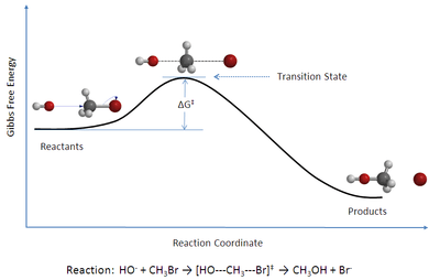
Rates of reaction can be studied by examining activated complexes near the saddle point of a potential energy surface. The details of how these complexes are formed are not important. The saddle point itself is called the transition state.
The activated complexes are in a special equilibrium (quasi-equilibrium) with the reactant molecules.
The activated complexes can convert into products, and kinetic theory can be used to calculate the rate of this conversion.

Development

In the development of TST, three approaches were taken as summarized below

Thermodynamic treatment

In 1884, Jacobus van't Hoff proposed the Van 't Hoff equation describing the temperature dependence of the equilibrium constant for a reversible reaction:

A ⇌ B

{\frac {d\ln K}{dT}}={\frac {\Delta U}{RT^{2}}}

where ΔU is the change in internal energy, K is the equilibrium constant of the reaction, R is the universal gas constant, and T is thermodynamic temperature. Based on experimental work, in 1889, Svante Arrhenius proposed a similar expression for the rate constant of a reaction, given as follows:

{\frac {d\ln k}{dT}}={\frac {\Delta E}{RT^{2}}}

Integration of this expression leads to the Arrhenius equation

k=Ae^{-E_{a}/RT}

where k is the rate constant. A was referred to as the frequency factor (now called the pre-exponential coefficient), and E_a is regarded as the activation energy. By the early 20th century many had accepted the Arrhenius equation, but the physical interpretation of A and E_a remained vague. This led many researchers in chemical kinetics to offer different theories of how chemical reactions occurred in an attempt to relate A and E_a to the molecular dynamics directly responsible for chemical reactions.

In 1910, French chemist René Marcelin introduced the concept of standard Gibbs energy of activation. His relation can be written as

k\propto \exp \left({\frac {-\Delta ^{\ddagger }G^{\ominus }}{RT}}\right)

At about the same time as Marcelin was working on his formulation, Dutch chemists Philip Abraham Kohnstamm, Frans Eppo Cornelis Scheffer, and Wiedold Frans Brandsma introduced standard entropy of activation and the standard enthalpy of activation. They proposed the following rate constant equation

k\propto \exp \left({\frac {\Delta ^{\ddagger }S^{\ominus }}{R}}\right)\exp \left({\frac {-\Delta ^{\ddagger }H^{\ominus }}{RT}}\right)

However, the nature of the constant was still unclear.

Kinetic-theory treatment

In early 1900, Max Trautz and William Lewis studied the rate of the reaction using collision theory, based on the kinetic theory of gases. Collision theory treats reacting molecules as hard spheres colliding with one another; this theory neglects entropy changes, since it assumes that the collision between molecules are completely elastic.

Lewis applied his treatment to the following reaction and obtained good agreement with experimental result.

2HI → H₂ + I₂

However, later when the same treatment was applied to other reactions, there were large discrepancies between theoretical and experimental results.

Statistical-mechanical treatment

Statistical mechanics played a significant role in the development of TST. However, the application of statistical mechanics to TST was developed very slowly given the fact that in mid-19th century, James Clerk Maxwell, Ludwig Boltzmann, and Leopold Pfaundler published several papers discussing reaction equilibrium and rates in terms of molecular motions and the statistical distribution of molecular speeds.

It was not until 1912 when the French chemist A. Berthoud used the Maxwell–Boltzmann distribution law to obtain an expression for the rate constant.

{\frac {d\ln k}{dT}}={\frac {a-bT}{RT^{2}}}

where a and b are constants related to energy terms.

Two years later, René Marcelin made an essential contribution by treating the progress of a chemical reaction as a motion of a point in phase space. He then applied Gibbs' statistical-mechanical procedures and obtained an expression similar to the one he had obtained earlier from thermodynamic consideration.

In 1915, another important contribution came from British physicist James Rice. Based on his statistical analysis, he concluded that the rate constant is proportional to the "critical increment". His ideas were further developed by Richard Chace Tolman. In 1919, Austrian physicist Karl Ferdinand Herzfeld applied statistical mechanics to the equilibrium constant and kinetic theory to the rate constant of the reverse reaction, k₋₁, for the reversible dissociation of a diatomic molecule.^[7]

{\ce {AB <=>[k_1][k_{-1}] {A}+ {B}}}

He obtained the following equation for the rate constant of the forward reaction^[8]

k_{1}={\frac {k_{\mathrm {B} }T}{h}}\left(1-e^{-{\frac {h\nu }{k_{B}T}}}\right)\exp \left({\frac {-E^{\ominus }}{RT}}\right)

where $\textstyle E^{\ominus }$ is the dissociation energy at absolute zero, k_B is the Boltzmann constant, h is the Planck constant, T is thermodynamic temperature, υ is vibrational frequency of the bond. This expression is very important since it is the first time that the factor k_BT/h, which is a critical component of TST, has appeared in a rate equation.

In 1920, the American chemist Richard Chace Tolman further developed Rice's idea of the critical increment. He concluded that critical increment (now referred to as activation energy) of a reaction is equal to the average energy of all molecules undergoing reaction minus the average energy of all reactant molecules.

Potential energy surfaces

The concept of potential energy surface was very important in the development of TST. The foundation of this concept was laid by René Marcelin in 1913. He theorized that the progress of a chemical reaction could be described as a point in a potential energy surface with coordinates in atomic momenta and distances.

In 1931, Henry Eyring and Michael Polanyi constructed a potential energy surface for the reaction below. This surface is a three-dimensional diagram based on quantum-mechanical principles as well as experimental data on vibrational frequencies and energies of dissociation.

H + H₂ → H₂ + H

A year after the Eyring and Polanyi construction, Hans Pelzer and Eugene Wigner made an important contribution by following the progress of a reaction on a potential energy surface. The importance of this work was that it was the first time that the concept of col or saddle point in the potential energy surface was discussed. They concluded that the rate of a reaction is determined by the motion of the system through that col.

It has been typically assumed that the rate-limiting or lowest saddle point is located on the same energy surface as the initial ground state. However, it was recently found that this could be incorrect for processes occurring in semiconductors and insulators, where an initial excited state could go through a saddle point lower than the one on the surface of the initial ground state.^[9]

Derivation of the Eyring equation

One of the most important features introduced by Eyring, Polanyi and Evans was the notion that activated complexes are in quasi-equilibrium with the reactants. The rate is then directly proportional to the concentration of these complexes multiplied by the frequency (k_BT/h) with which they are converted into products.

Quasi-equilibrium assumption

It should be noted that quasi-equilibrium is different from classical chemical equilibrium, but can be described using the same thermodynamic treatment.^[5] Consider the reaction below

{\ce {{A}+{B}<=>{[AB]^{\ddagger }}->{P}}}

Figure 2: Potential energy diagram

where complete equilibrium is achieved between all the species in the system including activated complexes, [AB]^‡ . Using statistical mechanics, concentration of [AB]^‡ can be calculated in terms of the concentration of A and B.

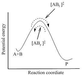
TST assumes that even when the reactants and products are not in equilibrium with each other, the activated complexes are in quasi-equilibrium with the reactants. As illustrated in Figure 2, at any instant of time, there are a few activated complexes, and some were reactant molecules in the immediate past, which are designated [AB_l]^‡ (since they are moving from left to right). The remainder of them were product molecules in the immediate past ([AB_r]^‡). Since the system is in complete equilibrium, the concentrations of [AB_l] ^‡ and [AB_r]^‡ are equal, so that each concentration is equal to one-half of the total concentration of activated complexes:

[{\ce {AB}}_{r}]^{\ddagger }=[{\ce {AB}}_{l}]^{\ddagger }={\frac {1}{2}}[{\ce {AB}}]^{\ddagger }

In TST, it is assumed that the flux of activated complexes in the two directions are independent of each other. That is, if all the product molecules were suddenly removed from the reaction system, the flow of [AB_r]^‡ stops, but there is still a flow from left to right. Hence, to be technically correct, the reactants are in equilibrium only with [AB_l]^‡, the activated complexes that were reactants in the immediate past.

The activated complexes do not follow a Boltzmann distribution of energies, but an "equilibrium constant" can still be derived from the distribution they do follow. The equilibrium constant K^‡ɵ for the quasi-equilibrium can be written as

K^{\ddagger \ominus }={\frac {\ce {[AB]^{\ddagger }}}{\ce {[A][B]}}}

So, the concentration of the transition state AB^‡ is

[{\ce {AB}}]^{\ddagger }=K^{\ddagger \ominus }[{\ce {A}}][{\ce {B}}]

Therefore, the rate equation for the production of product is

{\frac {d[{\ce {P}}]}{dt}}=k^{\ddagger \ominus }[{\ce {AB}}]^{\ddagger }=k^{\ddagger }K^{\ddagger }[{\ce {A}}][{\ce {B}}]=k[{\ce {A}}][{\ce {B}}]

Where the rate constant k is given by

k=k^{\ddagger }K^{\ddagger }

k^‡ is directly proportional to the frequency of the vibrational mode responsible for converting the activated complex to the product; the frequency of this vibrational mode is $\nu$ . Every vibration does not necessarily lead to the formation of product, so a proportionality constant $\kappa$ , referred to as the transmission coefficient, is introduced to account for this effect. So k^‡ can be rewritten as

k^{\ddagger }=\kappa \nu

For the equilibrium constant K^‡, statistical mechanics leads to a temperature dependent expression given as

K^{\ddagger }={\frac {k_{B}T}{h\nu }}K^{\ddagger '}

where

K^{\ddagger '}=e^{\frac {-\Delta G^{\ddagger }}{RT}}

Combining the new expressions for k^‡ and K^‡, a new rate constant expression can be written, which is given as

k=k^{\ddagger }K^{\ddagger }=\kappa {\frac {k_{B}T}{h}}e^{\frac {-\Delta G^{\ddagger }}{RT}}

Since, by definition, ΔG^‡ = ΔH^‡ –TΔS^‡, the rate constant expression can be expanded, to give an alternative form of the Eyring equation

k=\kappa {\frac {k_{B}T}{h}}e^{\frac {\Delta S^{\ddagger }}{R}}e^{\frac {-\Delta H^{\ddagger }}{RT}}

TST's rate constant expression can be used to calculate the Δ^‡G^ɵ, Δ^‡H^ɵ, Δ^‡S^ɵ, and even Δ^‡V (the volume of activation) using experimental rate data.

Given the relationship between equilibrium constant and the forward and reverse rate constants, $K=k_{1}/k_{-1}$ , the Eyring equation implies that

\Delta G^{\circ }=\Delta G_{1}^{\ddagger }-\Delta G_{-1}^{\ddagger }

Limitations of transition state theory

In general, TST has provided researchers with a conceptual foundation for understanding how chemical reactions take place. Even though the theory is widely applicable, it does have limitations. For example, when applied to each elementary step of a multi-step reaction, the theory assumes that each intermediate is long-lived enough to reach a Boltzmann distribution of energies before continuing to the next step. When the intermediates are very short-lived, TST fails. In such cases, the momentum of the reaction trajectory from the reactants to the intermediate can carry forward to affect product selectivity (an example of such a reaction is the thermal decomposition of diazaobicyclopentanes, presented by Anslyn and Dougherty).

Transition state theory is also based on the assumption that atomic nuclei behave according to classic mechanics.^[10] It is assumed that unless atoms or molecules collide with enough energy to form the transition structure, then the reaction does not occur. However, according to quantum mechanics, for any barrier with a finite amount of energy, there is a possibility that particles can still tunnel across the barrier. With respect to chemical reactions this means that there is a chance that molecules will react, even if they do not collide with enough energy to traverse the energy barrier.^[11] While this effect is negligible for reactions with large activation energies, it becomes an important phenomenon for reactions with relatively low energy barriers, since the tunneling probability increases with decreasing barrier height.

Transition state theory fails for some reactions at high temperature. The theory assumes the reaction system will pass over the lowest energy saddle point on the potential energy surface. While this description is consistent for reactions occurring at relatively low temperatures, at high temperatures, molecules populate higher energy vibrational modes; their motion becomes more complex and collisions may lead to transition states far away from the lowest energy saddle point. This deviation from transition state theory is observed even in the simple exchange reaction between diatomic hydrogen and a hydrogen radical.^[12]

Given these limitations, several alternatives to transition state theory have been proposed. A brief discussion of these theories follows.

Generalized transition state theory

Any form of TST, such as microcanonical variational TST, canonical variational TST, and improved canonical variational TST, in which the transition state is not necessarily located at the saddle point, is referred to as generalized transition state theory.

Microcanonical variational TST

A fundamental flaw of transition state theory is that it counts any crossing of the transition state as a reaction from reactants to products or vice versa. In reality, a molecule may cross this "dividing surface" and turn around, or cross multiple times and only truly react once. As such, unadjusted TST is said to provide an upper bound for the rate coefficients. To correct for this, variational transition state theory varies the location of the dividing surface that defines a successful reaction in order to minimize the rate for each fixed energy. ^[13] The rate expressions obtained in this microcanonical treatment can be integrated over the energy, taking into account the statistical distribution over energy states, so as to give the canonical, or thermal rates.

Canonical variational TST

A development of transition state theory in which the position of the dividing surface is varied so as to minimize the rate constant at a given temperature.

Improved canonical variational TST

A modification of canonical variational transition state theory in which, for energies below the threshold energy, the position of the dividing surface is taken to be that of the microcanonical threshold energy. This forces the contributions to rate constants to be zero if they are below the threshold energy. A compromise dividing surface is then chosen so as to minimize the contributions to the rate constant made by reactants having higher energies.

Nonadiabatic TST

An expansion of TST to the reactions when two spin-states are involved simultaneously is called nonadiabatic transition state theory (NA-TST).

Applications of TST: enzymatic reactions

Enzymes catalyze chemical reactions at rates that are astounding relative to uncatalyzed chemistry at the same reaction conditions. Each catalytic event requires a minimum of three or often more steps, all of which occur within the few milliseconds that characterize typical enzymatic reactions. According to transition state theory, the smallest fraction of the catalytic cycle is spent in the most important step, that of the transition state. The original proposals of absolute reaction rate theory for chemical reactions defined the transition state as a distinct species in the reaction coordinate that determined the absolute reaction rate. Soon thereafter, Linus Pauling proposed that the powerful catalytic action of enzymes could be explained by specific tight binding to the transition state species ^[14] Because reaction rate is proportional to the fraction of the reactant in the transition state complex, the enzyme was proposed to increase the concentration of the reactive species.

This proposal was formalized by Wolfenden and coworkers at University of North Carolina at Chapel Hill, who hypothesized that the rate increase imposed by enzymes is proportional to the affinity of the enzyme for the transition state structure relative to the Michaelis complex.^[15] Because enzymes typically increase the non-catalyzed reaction rate by factors of 10¹⁰-10¹⁵, and Michaelis complexes often have dissociation constants in the range of 10⁻³-10⁻⁶ M, it is proposed that transition state complexes are bound with dissociation constants in the range of 10⁻¹⁴-10⁻²³ M. As substrate progresses from the Michaelis complex to product, chemistry occurs by enzyme-induced changes in electron distribution in the substrate.

Enzymes alter the electronic structure by protonation, proton abstraction, electron transfer, geometric distortion, hydrophobic partitioning, and interaction with Lewis acids and bases. These are accomplished by sequential protein and substrate conformational changes. When a combination of individually weak forces are brought to bear on the substrate, the summation of the individual energies results in large forces capable of relocating bonding electrons to cause bond-breaking and bond-making. Analogs that resemble the transition state structures should therefore provide the most powerful noncovalent inhibitors known, even if only a small fraction of the transition state energy is captured.

All chemical transformations pass through an unstable structure called the transition state, which is poised between the chemical structures of the substrates and products. The transition states for chemical reactions are proposed to have lifetimes near 10⁻¹³ seconds, on the order of the time of a single bond vibration. No physical or spectroscopic method is available to directly observe the structure of the transition state for enzymatic reactions, yet transition state structure is central to understanding enzyme catalysis since enzymes work by lowering the activation energy of a chemical transformation.

It is now accepted that enzymes function to stabilize transition states lying between reactants and products, and that they would therefore be expected to bind strongly any inhibitor that closely resembles such a transition state. Substrates and products often participate in several enzyme reactions, whereas the transition state tends to be characteristic of one particular enzyme, so that such an inhibitor tends to be specific for that particular enzyme. The identification of numerous transition state inhibitors supports the transition state stabilization hypothesis for enzymatic catalysis.

Currently there is a large number of enzymes known to interact with transition state analogs, most of which have been designed with the intention of inhibiting the target enzyme. Examples include HIV-1 protease, racemases, β-lactamases, metalloproteinases, cyclooxygenases and many others.

Notes

↑ IUPAC, Compendium of Chemical Terminology, 2nd ed. (the "Gold Book") (1997). Online corrected version: (2006–) "transition state theory".
↑ Truhlar, D. G.; Garrett, B. C.; Klippenstein, S. J. (1996). "Current Status of Transition-State Theory". J. Phys. Chem. 100 (31): 12771–12800. doi:10.1021/jp953748q.
↑ Laidler, K.; King, C. (1983). "Development of transition-state theory". J. Phys. Chem. 87 (15): 2657. doi:10.1021/j100238a002.
↑ Laidler, K.; King, C. (1998). "A lifetime of transition-state theory". The Chemical Intelligencer. 4 (3): 39.
1 2 Laidler, K. J. (1969). Theories of Chemical Reaction Rates. McGraw-Hill.
↑ Anslyn, E. V.; Dougherty, D. A. (2006). "Transition State Theory and Related Topics". Modern Physical Organic Chemistry. University Science Books. pp. 365–373. ISBN 1891389319.
↑ Herzfeld, K. E. (1919). "Zur Theorie der Reaktionsgeschwindigkeiten in Gasen". Annalen der Physik. 364 (15): 635–667. Bibcode:1919AnP...364..635H. doi:10.1002/andp.19193641504.
↑ Keith J. Laidler, Chemical Kinetics (3rd ed., Harper & Row 1987), p.277 ISBN 0-06-043862-2
↑ Luo, G.; Kuech, T. F.; Morgan, D. (2018). "Transition state redox during dynamical processes in semiconductors and insulators". NPG Asia Materials. 10. arXiv:1712.01686. Bibcode:2018npjAM..10...45L. doi:10.1038/s41427-018-0010-0.
↑ Eyring, H. (1935). "The Activated Complex in Chemical Reactions". J. Chem. Phys. 3 (2): 107–115. Bibcode:1935JChPh...3..107E. doi:10.1063/1.1749604.
↑ Masel, R. (1996). Principles of Adsorption and Reactions on Solid Surfaces. New York: Wiley.
↑ Pineda, J. R.; Schwartz, S. D. (2006). "Protein dynamics and catalysis: The problems of transition state theory and the subtlety of dynamic control". Phil. Trans. R. Soc. B. 361 (1472): 1433–1438. doi:10.1098/rstb.2006.1877. PMC 1647311. PMID 16873129.
↑ Truhlar, D.; Garrett, B. (1984). "Variational Transition State Theory". Annu. Rev. Phys. Chem. 35: 159–189. Bibcode:1984ARPC...35..159T. doi:10.1146/annurev.pc.35.100184.001111.
↑ Pauling, L. (1948). "Chemical Achievement and Hope for the Future". American Scientist. 36: 50–58.
↑ Radzicka, A.; Wolfenden, R. (1995). "A proficient enzyme". Science. 267 (5194): 90–93. Bibcode:1995Sci...267...90R. doi:10.1126/science.7809611. PMID 7809611.

References

Anslyn, Eric V.; Doughtery, Dennis A., Transition State Theory and Related Topics. In Modern Physical Organic Chemistry University Science Books: 2006; pp 365–373
Cleland, W.W., Isotope Effects: Determination of Enzyme Transition State Structure. Methods in Enzymology 1995, 249, 341-373
Laidler, K.; King, C., Development of transition-state theory. The Journal of Physical Chemistry 1983, 87, (15), 2657
Laidler, K., A lifetime of transition-state theory. The Chemical Intelligencer 1998, 4, (3), 39
Radzicka, A.; Woldenden, R., Transition State and Multisubstrate$Analog Inhibitors. Methods in Enzymology 1995, 249, 284-312
Schramm, VL., Enzymatic Transition States and Transition State Analog Design. Annual Review of Biochemistry 1998, 67, 693-720
Schramm, V.L., Enzymatic Transition State Theory and Transition State Analogue Design. Journal of Biological Chemistry 2007, 282, (39), 28297-28300

External links

Simple application of TST

This article is issued from Wikipedia. The text is licensed under Creative Commons - Attribution - Sharealike. Additional terms may apply for the media files.

[1] IUPAC, Compendium of Chemical Terminology, 2nd ed. (the "Gold Book") (1997). Online corrected version: (2006–) "transition state theory".

[2] Truhlar, D. G.; Garrett, B. C.; Klippenstein, S. J. (1996). "Current Status of Transition-State Theory". J. Phys. Chem. 100 (31): 12771–12800. doi:10.1021/jp953748q.

[3] Laidler, K.; King, C. (1983). "Development of transition-state theory". J. Phys. Chem. 87 (15): 2657. doi:10.1021/j100238a002.

[4] Laidler, K.; King, C. (1998). "A lifetime of transition-state theory". The Chemical Intelligencer. 4 (3): 39.

[laidler-5] 1 2 Laidler, K. J. (1969). Theories of Chemical Reaction Rates. McGraw-Hill.

[6] Anslyn, E. V.; Dougherty, D. A. (2006). "Transition State Theory and Related Topics". Modern Physical Organic Chemistry. University Science Books. pp. 365–373. ISBN 1891389319.

[7] Herzfeld, K. E. (1919). "Zur Theorie der Reaktionsgeschwindigkeiten in Gasen". Annalen der Physik. 364 (15): 635–667. Bibcode:1919AnP...364..635H. doi:10.1002/andp.19193641504.

[8] Keith J. Laidler, Chemical Kinetics (3rd ed., Harper & Row 1987), p.277 ISBN 0-06-043862-2

[9] Luo, G.; Kuech, T. F.; Morgan, D. (2018). "Transition state redox during dynamical processes in semiconductors and insulators". NPG Asia Materials. 10. arXiv:1712.01686. Bibcode:2018npjAM..10...45L. doi:10.1038/s41427-018-0010-0.

[10] Eyring, H. (1935). "The Activated Complex in Chemical Reactions". J. Chem. Phys. 3 (2): 107–115. Bibcode:1935JChPh...3..107E. doi:10.1063/1.1749604.

[11] Masel, R. (1996). Principles of Adsorption and Reactions on Solid Surfaces. New York: Wiley.

[12] Pineda, J. R.; Schwartz, S. D. (2006). "Protein dynamics and catalysis: The problems of transition state theory and the subtlety of dynamic control". Phil. Trans. R. Soc. B. 361 (1472): 1433–1438. doi:10.1098/rstb.2006.1877. PMC 1647311. PMID 16873129.

[Truhlar1984-13] Truhlar, D.; Garrett, B. (1984). "Variational Transition State Theory". Annu. Rev. Phys. Chem. 35: 159–189. Bibcode:1984ARPC...35..159T. doi:10.1146/annurev.pc.35.100184.001111.

[14] Pauling, L. (1948). "Chemical Achievement and Hope for the Future". American Scientist. 36: 50–58.

[15] Radzicka, A.; Wolfenden, R. (1995). "A proficient enzyme". Science. 267 (5194): 90–93. Bibcode:1995Sci...267...90R. doi:10.1126/science.7809611. PMID 7809611.