Receiver operating characteristic

ROC curve of three predictors of peptide cleaving in the proteasome.

A receiver operating characteristic curve, i.e., ROC curve, is a graphical plot that illustrates the diagnostic ability of a binary classifier system as its discrimination threshold is varied.

The ROC curve is created by plotting the true positive rate (TPR) against the false positive rate (FPR) at various threshold settings. The true-positive rate is also known as sensitivity, recall or probability of detection^[1] in machine learning. The false-positive rate is also known as the fall-out or probability of false alarm^[1] and can be calculated as (1 − specificity). It can also be thought of as a plot of the Power as a function of the Type I Error of the decision rule (when the performance is calculated from just a sample of the population, it can be thought of as estimators of these quantities). The ROC curve is thus the sensitivity as a function of fall-out. In general, if the probability distributions for both detection and false alarm are known, the ROC curve can be generated by plotting the cumulative distribution function (area under the probability distribution from $-\infty$ to the discrimination threshold) of the detection probability in the y-axis versus the cumulative distribution function of the false-alarm probability on the x-axis.

ROC analysis provides tools to select possibly optimal models and to discard suboptimal ones independently from (and prior to specifying) the cost context or the class distribution. ROC analysis is related in a direct and natural way to cost/benefit analysis of diagnostic decision making.

The ROC curve was first developed by electrical engineers and radar engineers during World War II for detecting enemy objects in battlefields and was soon introduced to psychology to account for perceptual detection of stimuli. ROC analysis since then has been used in medicine, radiology, biometrics, forecasting of natural hazards,^[2] meteorology,^[3] model performance assessment,^[4] and other areas for many decades and is increasingly used in machine learning and data mining research.

The ROC is also known as a relative operating characteristic curve, because it is a comparison of two operating characteristics (TPR and FPR) as the criterion changes.^[5]

Basic concept

A classification model (classifier or diagnosis) is a mapping of instances between certain classes/groups. The classifier or diagnosis result can be a real value (continuous output), in which case the classifier boundary between classes must be determined by a threshold value (for instance, to determine whether a person has hypertension based on a blood pressure measure). Or it can be a discrete class label, indicating one of the classes.

Let us consider a two-class prediction problem (binary classification), in which the outcomes are labeled either as positive (p) or negative (n). There are four possible outcomes from a binary classifier. If the outcome from a prediction is p and the actual value is also p, then it is called a true positive (TP); however if the actual value is n then it is said to be a false positive (FP). Conversely, a true negative (TN) has occurred when both the prediction outcome and the actual value are n, and false negative (FN) is when the prediction outcome is n while the actual value is p.

To get an appropriate example in a real-world problem, consider a diagnostic test that seeks to determine whether a person has a certain disease. A false positive in this case occurs when the person tests positive, but does not actually have the disease. A false negative, on the other hand, occurs when the person tests negative, suggesting they are healthy, when they actually do have the disease.

Let us define an experiment from P positive instances and N negative instances for some condition. The four outcomes can be formulated in a 2×2 contingency table or confusion matrix, as follows:

		True condition
	Total population	Condition positive	Condition negative	Prevalence = Σ Condition positive/Σ Total population	Accuracy (ACC) = Σ True positive + Σ True negative/Σ Total population
Predicted condition	Predicted condition positive	True positive, Power	False positive, Type I error	Positive predictive value (PPV), Precision = Σ True positive/Σ Predicted condition positive	False discovery rate (FDR) = Σ False positive/Σ Predicted condition positive
	Predicted condition negative	False negative, Type II error	True negative	False omission rate (FOR) = Σ False negative/Σ Predicted condition negative	Negative predictive value (NPV) = Σ True negative/Σ Predicted condition negative
		True positive rate (TPR), Recall, Sensitivity, probability of detection = Σ True positive/Σ Condition positive	False positive rate (FPR), Fall-out, probability of false alarm = Σ False positive/Σ Condition negative	Positive likelihood ratio (LR+) = TPR/FPR	Diagnostic odds ratio (DOR) = LR+/LR−	F₁ score = 2/1/Recall + 1/Precision
		False negative rate (FNR), Miss rate = Σ False negative/Σ Condition positive	Specificity (SPC), Selectivity, True negative rate (TNR) = Σ True negative/Σ Condition negative	Negative likelihood ratio (LR−) = FNR/TNR

ROC space

The ROC space and plots of the four prediction examples.

The contingency table can derive several evaluation "metrics" (see infobox). To draw a ROC curve, only the true positive rate (TPR) and false positive rate (FPR) are needed (as functions of some classifier parameter). The TPR defines how many correct positive results occur among all positive samples available during the test. FPR, on the other hand, defines how many incorrect positive results occur among all negative samples available during the test.

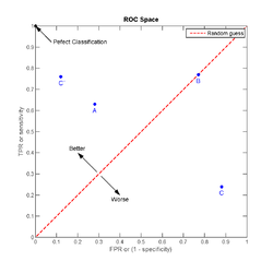
A ROC space is defined by FPR and TPR as x and y axes, respectively, which depicts relative trade-offs between true positive (benefits) and false positive (costs). Since TPR is equivalent to sensitivity and FPR is equal to 1 − specificity, the ROC graph is sometimes called the sensitivity vs (1 − specificity) plot. Each prediction result or instance of a confusion matrix represents one point in the ROC space.

The best possible prediction method would yield a point in the upper left corner or coordinate (0,1) of the ROC space, representing 100% sensitivity (no false negatives) and 100% specificity (no false positives). The (0,1) point is also called a perfect classification. A random guess would give a point along a diagonal line (the so-called line of no-discrimination) from the left bottom to the top right corners (regardless of the positive and negative base rates). An intuitive example of random guessing is a decision by flipping coins. As the size of the sample increases, a random classifier's ROC point tends towards the diagonal line. In the case of a balanced coin, it will tend to the point (0.5, 0.5).

The diagonal divides the ROC space. Points above the diagonal represent good classification results (better than random); points below the line represent bad results (worse than random). Note that the output of a consistently bad predictor could simply be inverted to obtain a good predictor.

Let us look into four prediction results from 100 positive and 100 negative instances:

A

B

C

C′

TP=63	FP=28	91
FN=37	TN=72	109
100	100	200

TP=77	FP=77	154
FN=23	TN=23	46
100	100	200

TP=24	FP=88	112
FN=76	TN=12	88
100	100	200

TP=76	FP=12	88
FN=24	TN=88	112
100	100	200

TPR = 0.63

TPR = 0.77

TPR = 0.24

TPR = 0.76

FPR = 0.28

FPR = 0.77

FPR = 0.88

FPR = 0.12

PPV = 0.69

PPV = 0.50

PPV = 0.21

PPV = 0.86

F1 = 0.66

F1 = 0.61

F1 = 0.23

F1 = 0.81

ACC = 0.68

ACC = 0.50

ACC = 0.18

ACC = 0.82

Plots of the four results above in the ROC space are given in the figure. The result of method A clearly shows the best predictive power among A, B, and C. The result of B lies on the random guess line (the diagonal line), and it can be seen in the table that the accuracy of B is 50%. However, when C is mirrored across the center point (0.5,0.5), the resulting method C′ is even better than A. This mirrored method simply reverses the predictions of whatever method or test produced the C contingency table. Although the original C method has negative predictive power, simply reversing its decisions leads to a new predictive method C′ which has positive predictive power. When the C method predicts p or n, the C′ method would predict n or p, respectively. In this manner, the C′ test would perform the best. The closer a result from a contingency table is to the upper left corner, the better it predicts, but the distance from the random guess line in either direction is the best indicator of how much predictive power a method has. If the result is below the line (i.e. the method is worse than a random guess), all of the method's predictions must be reversed in order to utilize its power, thereby moving the result above the random guess line.

Curves in ROC space

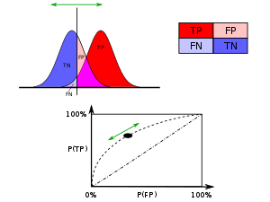
In binary classification, the class prediction for each instance is often made based on a continuous random variable $X$ , which is a "score" computed for the instance (e.g. the estimated probability in logistic regression). Given a threshold parameter $T$ , the instance is classified as "positive" if $X>T$ , and "negative" otherwise. $X$ follows a probability density $f_{1}(x)$ if the instance actually belongs to class "positive", and $f_{0}(x)$ if otherwise. Therefore, the true positive rate is given by ${\mbox{TPR}}(T)=\int _{T}^{\infty }f_{1}(x)\,dx$ and the false positive rate is given by ${\mbox{FPR}}(T)=\int _{T}^{\infty }f_{0}(x)\,dx$ . The ROC curve plots parametrically TPR(T) versus FPR(T) with T as the varying parameter.

For example, imagine that the blood protein levels in diseased people and healthy people are normally distributed with means of 2 g/dL and 1 g/dL respectively. A medical test might measure the level of a certain protein in a blood sample and classify any number above a certain threshold as indicating disease. The experimenter can adjust the threshold (black vertical line in the figure), which will in turn change the false positive rate. Increasing the threshold would result in fewer false positives (and more false negatives), corresponding to a leftward movement on the curve. The actual shape of the curve is determined by how much overlap the two distributions have. These concepts are demonstrated in the Receiver Operating Characteristic (ROC) Curves Applet.

Further interpretations

Sometimes, the ROC is used to generate a summary statistic. Common versions are:

the intercept of the ROC curve with the line at 45 degrees orthogonal to the no-discrimination line - the balance point where Sensitivity = Specificity
the intercept of the ROC curve with the tangent at 45 degrees parallel to the no-discrimination line that is closest to the error-free point (0,1) - also called Youden's J statistic and generalized as Informedness^[6]
the area between the ROC curve and the no-discrimination line multiplied by two - Gini Coefficient
the area between the full ROC curve and the triangular ROC curve including only (0,0), (1,1) and one selected operating point (tpr,fpr) - Consistency^[7]
the area under the ROC curve, or "AUC" ("Area Under Curve"), or A' (pronounced "a-prime"),^[8] or "c-statistic".^[9]
the sensitivity index d' (pronounced "d-prime"), the distance between the mean of the distribution of activity in the system under noise-alone conditions and its distribution under signal-alone conditions, divided by their standard deviation, under the assumption that both these distributions are normal with the same standard deviation. Under these assumptions, the shape of the ROC is entirely determined by d'.

However, any attempt to summarize the ROC curve into a single number loses information about the pattern of tradeoffs of the particular discriminator algorithm.

Area under the curve

When using normalized units, the area under the curve (often referred to as simply the AUC) is equal to the probability that a classifier will rank a randomly chosen positive instance higher than a randomly chosen negative one (assuming 'positive' ranks higher than 'negative').^[10] This can be seen as follows: the area under the curve is given by (the integral boundaries are reversed as large T has a lower value on the x-axis)

A=\int _{\infty }^{-\infty }{\mbox{TPR}}(T){\mbox{FPR}}'(T)\,dT=\int _{-\infty }^{\infty }\int _{-\infty }^{\infty }I(T'>T)f_{1}(T')f_{0}(T)\,dT'\,dT=P(X_{1}>X_{0})

where $X_{1}$ is the score for a positive instance and $X_{0}$ is the score for a negative instance, and $f_{0}$ and $f_{1}$ are probability densities as defined in previous section.

It can further be shown that the AUC is closely related to the Mann–Whitney U,^[11]^[12] which tests whether positives are ranked higher than negatives. It is also equivalent to the Wilcoxon test of ranks.^[12] The AUC is related to the Gini coefficient ( $G_{1}$ ) by the formula $G_{1}=2{\mbox{AUC}}-1$ , where:

G_{1}=1-\sum _{k=1}^{n}(X_{k}-X_{k-1})(Y_{k}+Y_{k-1})

^[13]

In this way, it is possible to calculate the AUC by using an average of a number of trapezoidal approximations.

It is also common to calculate the Area Under the ROC Convex Hull (ROC AUCH = ROCH AUC) as any point on the line segment between two prediction results can be achieved by randomly using one or other system with probabilities proportional to the relative length of the opposite component of the segment.^[14] It is also possible to invert concavities – just as in the figure the worse solution can be reflected to become a better solution; concavities can be reflected in any line segment, but this more extreme form of fusion is much more likely to overfit the data.^[15]

The machine learning community most often uses the ROC AUC statistic for model comparison.^[16] However, this practice has recently been questioned based upon new machine learning research that shows that the AUC is quite noisy as a classification measure^[17] and has some other significant problems in model comparison.^[18]^[19] A reliable and valid AUC estimate can be interpreted as the probability that the classifier will assign a higher score to a randomly chosen positive example than to a randomly chosen negative example. However, the critical research^[17]^[18] suggests frequent failures in obtaining reliable and valid AUC estimates. Thus, the practical value of the AUC measure has been called into question,^[19] raising the possibility that the AUC may actually introduce more uncertainty into machine learning classification accuracy comparisons than resolution. Nonetheless, the coherence of AUC as a measure of aggregated classification performance has been vindicated, in terms of a uniform rate distribution,^[20] and AUC has been linked to a number of other performance metrics such as the Brier score.^[21]

One recent explanation of the problem with ROC AUC is that reducing the ROC Curve to a single number ignores the fact that it is about the tradeoffs between the different systems or performance points plotted and not the performance of an individual system, as well as ignoring the possibility of concavity repair, so that related alternative measures such as Informedness^[6] or DeltaP are recommended.^[7]^[22] These measures are essentially equivalent to the Gini for a single prediction point with DeltaP' = Informedness = 2AUC-1, whilst DeltaP = Markedness represents the dual (viz. predicting the prediction from the real class) and their geometric mean is the Matthews correlation coefficient.^[6]

Whereas ROC AUC varies between 0 and 1 — with an uninformative classifier yielding 0.5 — the alternative measures known as Informedness^[6], Certainty ^[7] and Gini Coefficient (in the single parameterization or single system case)^[6] all have the advantage that 0 represents chance performance whilst 1 represents perfect performance, and −1 represents the "perverse" case of full informedness always giving the wrong response.^[23] Bringing chance performance to 0 allows these alternative scales to be interpreted as Kappa statistics. Informedness has been shown to have desirable characteristics for Machine Learning versus other common definitions of Kappa such as Cohen Kappa and Fleiss Kappa.^[6]^[24]

Sometimes it can be more useful to look at a specific region of the ROC Curve rather than at the whole curve. It is possible to compute partial AUC.^[25] For example, one could focus on the region of the curve with low false positive rate, which is often of prime interest for population screening tests.^[26] Another common approach for classification problems in which P ≪ N (common in bioinformatics applications) is to use a logarithmic scale for the x-axis.^[27]

Other measures

The Total Operating Characteristic (TOC) also characterizes diagnostic ability while revealing more information than the ROC. For each threshold, ROC reveals two ratios, TP/(TP + FN) and FP/(FP + TN). In other words, ROC reveals hits/(hits + misses)and false alarms/(false alarms + correct rejections). On the other hand, TOC shows the total information in the contingency table for each threshold.^[28] The TOC method reveals all of the information that the ROC method provides, plus additional important information that ROC does not reveal, i.e. the size of every entry in the contingency table for each threshold. TOC also provides the popular AUC of the ROC.

TOC Curve

ROC Curve

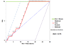
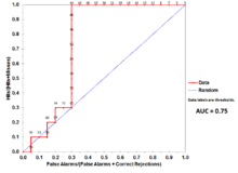
These figures are the TOC and ROC curves using the same data and thresholds. Consider the point that corresponds to a threshold of 74. The TOC curve shows the number of hits, which is 3, and hence the number of misses, which is 7. Additionally, the TOC curve shows that the number of false alarms is 4 and the number of correct rejections is 16. At any given point in the ROC curve, it is possible to glean values for the ratios of false alarms/(false alarms + correct rejections) and hits/(hits + misses). For example, at threshold 74, it is evident that the x coordinate is 0.3 and the y coordinate is 0.2. However, these two values are insufficient to construct all entries of the underlying two-by-two contingency table.

Detection error tradeoff graph

Example DET graph

An alternative to the ROC curve is the detection error tradeoff (DET) graph, which plots the false negative rate (missed detections) vs. the false positive rate (false alarms) on non-linearly transformed x- and y-axes. The transformation function is the quantile function of the normal distribution, i.e., the inverse of the cumulative normal distribution. It is, in fact, the same transformation as zROC, below, except that the complement of the hit rate, the miss rate or false negative rate, is used. This alternative spends more graph area on the region of interest. Most of the ROC area is of little interest; one primarily cares about the region tight against the y-axis and the top left corner – which, because of using miss rate instead of its complement, the hit rate, is the lower left corner in a DET plot. Furthermore, DET graphs have the useful property of linearity and a linear threshold behavior for normal distributions.^[29] The DET plot is used extensively in the automatic speaker recognition community, where the name DET was first used. The analysis of the ROC performance in graphs with this warping of the axes was used by psychologists in perception studies halfway through the 20th century, where this was dubbed "double probability paper".

Z-score

If a standard score is applied to the ROC curve, the curve will be transformed into a straight line.^[30] This z-score is based on a normal distribution with a mean of zero and a standard deviation of one. In memory strength theory, one must assume that the zROC is not only linear, but has a slope of 1.0. The normal distributions of targets (studied objects that the subjects need to recall) and lures (non studied objects that the subjects attempt to recall) is the factor causing the zROC to be linear.

The linearity of the zROC curve depends on the standard deviations of the target and lure strength distributions. If the standard deviations are equal, the slope will be 1.0. If the standard deviation of the target strength distribution is larger than the standard deviation of the lure strength distribution, then the slope will be smaller than 1.0. In most studies, it has been found that the zROC curve slopes constantly fall below 1, usually between 0.5 and 0.9.^[31] Many experiments yielded a zROC slope of 0.8. A slope of 0.8 implies that the variability of the target strength distribution is 25% larger than the variability of the lure strength distribution.^[32]

Another variable used is d' (d prime) (discussed above in "Other measures"), which can easily be expressed in terms of z-values. Although d' is a commonly used parameter, it must be recognized that it is only relevant when strictly adhering to the very strong assumptions of strength theory made above.^[33]

The z-score of an ROC curve is always linear, as assumed, except in special situations. The Yonelinas familiarity-recollection model is a two-dimensional account of recognition memory. Instead of the subject simply answering yes or no to a specific input, the subject gives the input a feeling of familiarity, which operates like the original ROC curve. What changes, though, is a parameter for Recollection (R). Recollection is assumed to be all-or-none, and it trumps familiarity. If there were no recollection component, zROC would have a predicted slope of 1. However, when adding the recollection component, the zROC curve will be concave up, with a decreased slope. This difference in shape and slope result from an added element of variability due to some items being recollected. Patients with anterograde amnesia are unable to recollect, so their Yonelinas zROC curve would have a slope close to 1.0.^[34]

History

The ROC curve was first used during World War II for the analysis of radar signals before it was employed in signal detection theory.^[35] Following the attack on Pearl Harbor in 1941, the United States army began new research to increase the prediction of correctly detected Japanese aircraft from their radar signals. For these purposes they measured the ability of a radar receiver operator to make these important distinctions, which was called the Receiver Operating Characteristic.^[36]

In the 1950s, ROC curves were employed in psychophysics to assess human (and occasionally non-human animal) detection of weak signals.^[35] In medicine, ROC analysis has been extensively used in the evaluation of diagnostic tests.^[37]^[38] ROC curves are also used extensively in epidemiology and medical research and are frequently mentioned in conjunction with evidence-based medicine. In radiology, ROC analysis is a common technique to evaluate new radiology techniques.^[39] In the social sciences, ROC analysis is often called the ROC Accuracy Ratio, a common technique for judging the accuracy of default probability models. ROC curves are widely used in laboratory medicine to assess the diagnostic accuracy of a test, to choose the optimal cut-off of a test and to compare diagnostic accuracy of several tests.

ROC curves also proved useful for the evaluation of machine learning techniques. The first application of ROC in machine learning was by Spackman who demonstrated the value of ROC curves in comparing and evaluating different classification algorithms.^[40]

ROC curves are also used in verification of forecasts in meteorology.^[41]

ROC curves beyond binary classification

The extension of ROC curves for classification problems with more than two classes has always been cumbersome, as the degrees of freedom increase quadratically with the number of classes, and the ROC space has $c(c-1)$ dimensions, where $c$ is the number of classes.^[42] Some approaches have been made for the particular case with three classes (three-way ROC).^[43] The calculation of the volume under the ROC surface (VUS) has been analyzed and studied as a performance metric for multi-class problems.^[44] However, because of the complexity of approximating the true VUS, some other approaches ^[45] based on an extension of AUC are more popular as an evaluation metric.

Given the success of ROC curves for the assessment of classification models, the extension of ROC curves for other supervised tasks has also been investigated. Notable proposals for regression problems are the so-called regression error characteristic (REC) Curves ^[46] and the Regression ROC (RROC) curves.^[47] In the latter, RROC curves become extremely similar to ROC curves for classification, with the notions of asymmetry, dominance and convex hull. Also, the area under RROC curves is proportional to the error variance of the regression model.

References

1 2 "Detector Performance Analysis Using ROC Curves - MATLAB & Simulink Example". www.mathworks.com. Retrieved 11 August 2016.
↑ Peres, D. J.; Cancelliere, A. (2014-12-08). "Derivation and evaluation of landslide-triggering thresholds by a Monte Carlo approach". Hydrol. Earth Syst. Sci. 18 (12): 4913–4931. Bibcode:2014HESS...18.4913P. doi:10.5194/hess-18-4913-2014. ISSN 1607-7938.
↑ Murphy, Allan H. (1996-03-01). "The Finley Affair: A Signal Event in the History of Forecast Verification". Weather and Forecasting. 11 (1): 3–20. doi:10.1175/1520-0434(1996)011<0003:tfaase>2.0.co;2. ISSN 0882-8156.
↑ Peres, D. J.; Iuppa, C.; Cavallaro, L.; Cancelliere, A.; Foti, E. (2015-10-01). "Significant wave height record extension by neural networks and reanalysis wind data". Ocean Modelling. 94: 128–140. Bibcode:2015OcMod..94..128P. doi:10.1016/j.ocemod.2015.08.002.
↑ Swets, John A.; Signal detection theory and ROC analysis in psychology and diagnostics : collected papers, Lawrence Erlbaum Associates, Mahwah, NJ, 1996
1 2 3 4 5 6 Powers, David M W (2011) [2007]. "Evaluation: From Precision, Recall and F-Measure to ROC, Informedness, Markedness & Correlation" (PDF). Journal of Machine Learning Technologies. 2 (1): 37–63.
1 2 3 Powers, David MW (2012). "ROC-ConCert: ROC-Based Measurement of Consistency and Certainty". Spring Congress on Engineering and Technology (SCET). 2. IEEE. pp. 238–241.
↑ Fogarty, James; Baker, Ryan S.; Hudson, Scott E. (2005). "Case studies in the use of ROC curve analysis for sensor-based estimates in human computer interaction". ACM International Conference Proceeding Series, Proceedings of Graphics Interface 2005. Waterloo, ON: Canadian Human-Computer Communications Society.
↑ Hastie, Trevor; Tibshirani, Robert; Friedman, Jerome H. (2009). The elements of statistical learning: data mining, inference, and prediction (2nd ed.).
↑ Fawcett, Tom (2006); An introduction to ROC analysis, Pattern Recognition Letters, 27, 861–874.
↑ Hanley, James A.; McNeil, Barbara J. (1982). "The Meaning and Use of the Area under a Receiver Operating Characteristic (ROC) Curve". Radiology. 143 (1): 29–36. doi:10.1148/radiology.143.1.7063747. PMID 7063747.
1 2 Mason, Simon J.; Graham, Nicholas E. (2002). "Areas beneath the relative operating characteristics (ROC) and relative operating levels (ROL) curves: Statistical significance and interpretation" (PDF). Quarterly Journal of the Royal Meteorological Society. 128: 2145–2166. doi:10.1256/003590002320603584. Archived from the original (PDF) on 2008-11-20.
↑ Hand, David J.; and Till, Robert J. (2001); A simple generalization of the area under the ROC curve for multiple class classification problems, Machine Learning, 45, 171–186.
↑ Provost, F.; Fawcett, T. (2001). "Robust classification for imprecise environments". Machine Learning. 42: 203–231. arXiv:cs/0009007. doi:10.1023/a:1007601015854.
↑ Flach, P.A.; Wu, S. (2005). "Repairing concavities in ROC curves." (PDF). 19th International Joint Conference on Artificial Intelligence (IJCAI'05). pp. 702–707.
↑ Hanley, James A.; McNeil, Barbara J. (1983-09-01). "A method of comparing the areas under receiver operating characteristic curves derived from the same cases". Radiology. 148 (3): 839–843. doi:10.1148/radiology.148.3.6878708. PMID 6878708. Retrieved 2008-12-03.
1 2 Hanczar, Blaise; Hua, Jianping; Sima, Chao; Weinstein, John; Bittner, Michael; Dougherty, Edward R (2010). "Small-sample precision of ROC-related estimates". Bioinformatics. 26 (6): 822–830. doi:10.1093/bioinformatics/btq037.
1 2 Lobo, Jorge M.; Jiménez-Valverde, Alberto; Real, Raimundo (2008). "AUC: a misleading measure of the performance of predictive distribution models". Global Ecology and Biogeography. 17: 145–151. doi:10.1111/j.1466-8238.2007.00358.x.
1 2 Hand, David J (2009). "Measuring classifier performance: A coherent alternative to the area under the ROC curve". Machine Learning. 77: 103–123. doi:10.1007/s10994-009-5119-5.
↑ Flach, P.A.; Hernandez-Orallo, J.; Ferri, C. (2011). "A coherent interpretation of AUC as a measure of aggregated classification performance." (PDF). Proceedings of the 28th International Conference on Machine Learning (ICML-11). pp. 657–664.
↑ Hernandez-Orallo, J.; Flach, P.A.; Ferri, C. (2012). "A unified view of performance metrics: translating threshold choice into expected classification loss" (PDF). Journal of Machine Learning Research. 13: 2813–2869.
↑ Powers, David M.W. (2012). "The Problem of Area Under the Curve". International Conference on Information Science and Technology.
↑ Powers, David M. W. (2003). "Recall and Precision versus the Bookmaker" (PDF). Proceedings of the International Conference on Cognitive Science (ICSC-2003), Sydney Australia, 2003, pp. 529–534.
↑ Powers, David M. W. (2012). "The Problem with Kappa" (PDF). Conference of the European Chapter of the Association for Computational Linguistics (EACL2012) Joint ROBUS-UNSUP Workshop.
↑ McClish, Donna Katzman (1989-08-01). "Analyzing a Portion of the ROC Curve". Medical Decision Making. 9 (3): 190–195. doi:10.1177/0272989X8900900307. PMID 2668680. Retrieved 2008-09-29.
↑ Dodd, Lori E.; Pepe, Margaret S. (2003). "Partial AUC Estimation and Regression". Biometrics. 59 (3): 614–623. doi:10.1111/1541-0420.00071. PMID 14601762. Retrieved 2007-12-18.
↑ Karplus, Kevin (2011); Better than Chance: the importance of null models, University of California, Santa Cruz, in Proceedings of the First International Workshop on Pattern Recognition in Proteomics, Structural Biology and Bioinformatics (PR PS BB 2011)
↑ Pontius, Robert Gilmore; Parmentier, Benoit (2014). "Recommendations for using the Relative Operating Characteristic (ROC)". Landscape Ecology.
↑ Navractil, J.; Klusacek, D. (2007-04-01). "On Linear DETs". 2007 IEEE International Conference on Acoustics, Speech and Signal Processing - ICASSP '07. 4: IV–229-IV-232. doi:10.1109/ICASSP.2007.367205.
↑ MacMillan, Neil A.; Creelman, C. Douglas (2005). Detection Theory: A User's Guide (2nd ed.). Mahwah, NJ: Lawrence Erlbaum Associates. ISBN 1-4106-1114-0.
↑ Glanzer, Murray; Kisok, Kim; Hilford, Andy; Adams, John K. (1999). "Slope of the receiver-operating characteristic in recognition memory". Journal of Experimental Psychology: Learning, Memory, and Cognition. 25 (2): 500–513. doi:10.1037/0278-7393.25.2.500.
↑ Ratcliff, Roger; McCoon, Gail; Tindall, Michael (1994). "Empirical generality of data from recognition memory ROC functions and implications for GMMs". Journal of Experimental Psychology: Learning, Memory, and Cognition. 20: 763–785. doi:10.1037/0278-7393.20.4.763.
↑ Zhang, Jun; Mueller, Shane T. (2005). "A note on ROC analysis and non-parametric estimate of sensitivity". Psychometrika. 70: 203–212. doi:10.1007/s11336-003-1119-8.
↑ Yonelinas, Andrew P.; Kroll, Neal E. A.; Dobbins, Ian G.; Lazzara, Michele; Knight, Robert T. (1998). "Recollection and familiarity deficits in amnesia: Convergence of remember-know, process dissociation, and receiver operating characteristic data". Neuropsychology. 12: 323–339. doi:10.1037/0894-4105.12.3.323.
1 2 Green, David M.; Swets, John A. (1966). Signal detection theory and psychophysics. New York, NY: John Wiley and Sons Inc. ISBN 0-471-32420-5.
↑ "Using the Receiver Operating Characteristic (ROC) curve to analyze a classification model: A final note of historical interest" (PDF). Department of Mathematics, University of Utah. Department of Mathematics, University of Utah. Retrieved May 25, 2017.
↑ Zweig, Mark H.; Campbell, Gregory (1993). "Receiver-operating characteristic (ROC) plots: a fundamental evaluation tool in clinical medicine" (PDF). Clinical Chemistry. 39 (8): 561–577. PMID 8472349.
↑ Pepe, Margaret S. (2003). The statistical evaluation of medical tests for classification and prediction. New York, NY: Oxford. ISBN 0-19-856582-8.
↑ Obuchowski, Nancy A. (2003). "Receiver operating characteristic curves and their use in radiology". Radiology. 229 (1): 3–8. doi:10.1148/radiol.2291010898. PMID 14519861.
↑ Spackman, Kent A. (1989). "Signal detection theory: Valuable tools for evaluating inductive learning". Proceedings of the Sixth International Workshop on Machine Learning. San Mateo, CA: Morgan Kaufmann. pp. 160–163.
↑ Kharin, Viatcheslav (2003). "On the ROC score of probability forecasts". Journal of Climate. 16 (24): 4145–4150. doi:10.1175/1520-0442(2003)016<4145:OTRSOP>2.0.CO;2.
↑ Srinivasan, A. (1999). "Note on the Location of Optimal Classifiers in N-dimensional ROC Space". Technical Report PRG-TR-2-99, Oxford University Computing Laboratory, Wolfson Building, Parks Road, Oxford.
↑ Mossman, D. (1999). "Three-way ROCs". Medical Decision Making. 19: 78–89. doi:10.1177/0272989x9901900110.
↑ Ferri, C.; Hernandez-Orallo, J.; Salido, M.A. (2003). "Volume under the ROC Surface for Multi-class Problems". Machine Learning: ECML 2003. pp. 108–120.
↑ Till, D.J.; Hand, R.J. (2012). "A Simple Generalisation of the Area Under the ROC Curve for Multiple Class Classification Problems". Machine Learning. 45: 171–186. doi:10.1023/A:1010920819831.
↑ Bi, J.; Bennett, K.P. (2003). "Regression error characteristic curves". Twentieth International Conference on Machine Learning (ICML-2003). Washington, DC.
↑ Hernandez-Orallo, J. (2013). "ROC curves for regression". Pattern Recognition. 46 (12): 3395–3411 . doi:10.1016/j.patcog.2013.06.014.
↑ Fawcett, Tom (2006). "An Introduction to ROC Analysis" (PDF). Pattern Recognition Letters. 27 (8): 861–874. doi:10.1016/j.patrec.2005.10.010.
↑ Powers, David M W (2011). "Evaluation: From Precision, Recall and F-Measure to ROC, Informedness, Markedness & Correlation" (PDF). Journal of Machine Learning Technologies. 2 (1): 37–63.
↑ Ting, Kai Ming (2011). Encyclopedia of machine learning. Springer. ISBN 978-0-387-30164-8.