Cross-correlation

Visual comparison of convolution, cross-correlation and autocorrelation. For the operations involving function

f

, and assuming the height of

f

is 1.0, the value of the result at 5 different points is indicated by the shaded area below each point. Also, the vertical symmetry of

f

is the reason

f*g

and

f\star g

are identical in this example.

In signal processing, cross-correlation is a measure of similarity of two series as a function of the displacement of one relative to the other. This is also known as a sliding dot product or sliding inner-product. It is commonly used for searching a long signal for a shorter, known feature. It has applications in pattern recognition, single particle analysis, electron tomography, averaging, cryptanalysis, and neurophysiology.

For continuous functions f and g, the cross-correlation is defined as:^[1]^[2]^[3]

(f\star g)(\tau )\ {\stackrel {\mathrm {def} }{=}}\int _{-\infty }^{\infty }f^{*}(t)\ g(t+\tau )\,dt

,

where $f^{*}$ denotes the complex conjugate of $f$ , and $\tau$ is the displacement, also known as lag (a feature in f at t occurs in g at $t+\tau$ ).

Similarly, for discrete functions, the cross-correlation is defined as:^[4]^[5]

(f\star g)[n]\ {\stackrel {\mathrm {def} }{=}}\sum _{m=-\infty }^{\infty }f^{*}[m]\ g[m+n].

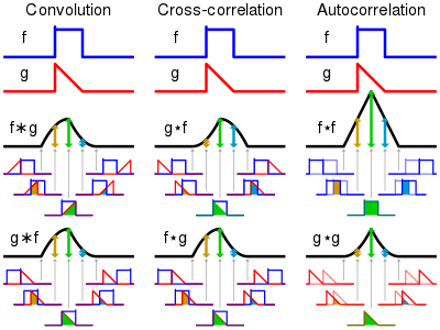
The cross-correlation is similar in nature to the convolution of two functions. In an autocorrelation, which is the cross-correlation of a signal with itself, there will always be a peak at a lag of zero, and its size will be the signal energy.

In probability and statistics, the term cross-correlations is used for referring to the correlations between the entries of two random vectors X and Y, while the correlations of a random vector X are considered to be the correlations between the entries of X itself, those forming the correlation matrix (matrix of correlations) of X. If each of X and Y is a scalar random variable which is realized repeatedly in temporal sequence (a time series), then the correlations of the various temporal instances of X are known as autocorrelations of X, and the cross-correlations of X with Y across time are temporal cross-correlations.

Furthermore, in probability and statistics the definition of correlation always includes a standardising factor in such a way that correlations have values between −1 and +1.

If $X$ and $Y$ are two independent random variables with probability density functions f and g, respectively, then the probability density of the difference $Y-X$ is formally given by the cross-correlation (in the signal-processing sense) $f\star g$ ; however this terminology is not used in probability and statistics. In contrast, the convolution $f*g$ (equivalent to the cross-correlation of f(t) and g(−t) ) gives the probability density function of the sum $X+Y$ .

Explanation

As an example, consider two real valued functions $f$ and $g$ differing only by an unknown shift along the x-axis. One can use the cross-correlation to find how much $g$ must be shifted along the x-axis to make it identical to $f$ . The formula essentially slides the $g$ function along the x-axis, calculating the integral of their product at each position. When the functions match, the value of $(f\star g)$ is maximized. This is because when peaks (positive areas) are aligned, they make a large contribution to the integral. Similarly, when troughs (negative areas) align, they also make a positive contribution to the integral because the product of two negative numbers is positive.

Animation displaying visually how cross correlation is calculated

With complex-valued functions $f$ and $g$ , taking the conjugate of $f$ ensures that aligned peaks (or aligned troughs) with imaginary components will contribute positively to the integral.

In econometrics, lagged cross-correlation is sometimes referred to as cross-autocorrelation.^[6]^{:p. 74}

Properties

The cross-correlation of functions f(t) and g(t) is equivalent to the convolution (denoted by $*$ ) of f^*(−t) and g(t). That is:
$[f(t)\star g(t)](t)=[f^{*}(-t)*g(t)](t).$
$[f(t)\star g(t)](t)=[g^{*}(t)\star f^{*}(t)](-t).$
If f is a Hermitian function, then $f\star g=f*g.$
If both f and g are Hermitian, then $f\star g=g\star f$ .
$\left(f\star g\right)\star \left(f\star g\right)=\left(f\star f\right)\star \left(g\star g\right)$ .
Analogous to the convolution theorem, the cross-correlation satisfies
${\mathcal {F}}\left\{f\star g\right\}={\mathcal {F}}\left\{f\right\}^{*}\cdot {\mathcal {F}}\left\{g\right\},$

where

{\mathcal {F}}

denotes the Fourier transform, and an asterisk again indicates the complex conjugate, since

{\mathcal {F}}\left\{f(-t)\right\}={\mathcal {F}}\left\{f(t)\right\}^{*}

. Coupled with fast Fourier transform algorithms, this property is often exploited for the efficient numerical computation of cross-correlations ^[7] (see circular cross-correlation).

The cross-correlation is related to the spectral density (see Wiener–Khinchin theorem).
The cross-correlation of a convolution of f and h with a function g is the convolution of the cross-correlation of g and f with the kernel h:
$g\star \left(f*h\right)=\left(g\star f\right)*h.$

Time series analysis

In time series analysis, as applied in statistics, the cross-correlation between two time series is the normalized cross-covariance function.

Let $(X_{t},Y_{t})$ represent a pair of stochastic processes that are jointly wide-sense stationary. Then the cross-covariance and the cross-correlation are given by

Cross-covariance: $\gamma _{XY}(\tau )=\operatorname {E} \left[\left(X_{t}-\mu _{X}\right)\left(Y_{t+\tau }-\mu _{Y}\right)\right],$
Cross correlation coefficient: $\rho _{XY}(\tau )={\frac {1}{\sigma _{X}\sigma _{Y}}}\operatorname {E} \left[\left(X_{t}-\mu _{X}\right)\left(Y_{t+\tau }-\mu _{Y}\right)\right]={\frac {1}{\sigma _{X}\sigma _{Y}}}\gamma _{XY}(\tau ),$

where $\mu _{X}$ and $\sigma _{X}$ are the mean and standard deviation of the process $(X_{t})$ , which are constant over time due to stationarity; and similarly for $(Y_{t})$ , respectively. $\operatorname {E} [\ ]$ indicates the expected value. That the cross-covariance and cross-correlation are independent of t is precisely the additional information (beyond being individually wide-sense stationary) conveyed by the requirement that $(X_{t},Y_{t})$ are jointly wide-sense stationary.

The cross-correlation of a pair of jointly wide sense stationary stochastic processes can be estimated by averaging the product of samples measured from one process and samples measured from the other (and its time shifts). The samples included in the average can be an arbitrary subset of all the samples in the signal (e.g., samples within a finite time window or a sub-sampling of one of the signals). For a large number of samples, the average converges to the true cross-correlation.

Time delay analysis

Cross-correlations are useful for determining the time delay between two signals, e.g. for determining time delays for the propagation of acoustic signals across a microphone array.^[8]^[9] After calculating the cross-correlation between the two signals, the maximum (or minimum if the signals are negatively correlated) of the cross-correlation function indicates the point in time where the signals are best aligned; i.e., the time delay between the two signals is determined by the argument of the maximum, or arg max of the cross-correlation, as in

\tau _{\mathrm {delay} }={\underset {t\in \mathbb {R} }{\operatorname {arg\,max} }}((f\star g)(t))

Zero-normalized cross-correlation (ZNCC)

For image-processing applications in which the brightness of the image and template can vary due to lighting and exposure conditions, the images can be first normalized. This is typically done at every step by subtracting the mean and dividing by the standard deviation. That is, the cross-correlation of a template, $t(x,y)$ with a subimage $f(x,y)$ is

{\frac {1}{n}}\sum _{x,y}{\frac {1}{\sigma _{f}\sigma _{t}}}\left(f(x,y)-{\overline {f}}\right)\left(t(x,y)-{\overline {t}}\right)

.

where $n$ is the number of pixels in $t(x,y)$ and $f(x,y)$ , ${\overline {f}}$ is the average of f and $\sigma _{f}$ is standard deviation of f.

In functional analysis terms, this can be thought of as the dot product of two normalized vectors. That is, if

F(x,y)=f(x,y)-{\overline {f}}

and

T(x,y)=t(x,y)-{\overline {t}}

then the above sum is equal to

\left\langle {\frac {F}{\|F\|}},{\frac {T}{\|T\|}}\right\rangle

where $\langle \cdot ,\cdot \rangle$ is the inner product and $\|\cdot \|$ is the L² norm.

Thus, if f and t are real matrices, their normalized cross-correlation equals the cosine of the angle between the unit vectors F and T, being thus 1 if and only if F equals T multiplied by a positive scalar.

Normalized correlation is one of the methods used for template matching, a process used for finding incidences of a pattern or object within an image. It is also the 2-dimensional version of Pearson product-moment correlation coefficient.

Normalized cross-correlation (NCC)

NCC is similar to ZNCC with the only difference of not subtracting the local mean value of intensities.

Nonlinear systems

Caution must be applied when using cross correlation for nonlinear systems. In certain circumstances, which depend on the properties of the input, cross correlation between the input and output of a system with nonlinear dynamics can be completely blind to certain nonlinear effects.^[10] This problem arises because some quadratic moments can equal zero and this can incorrectly suggest that there is little "correlation" (in the sense of statistical dependence) between two signals, when in fact the two signals are strongly related by nonlinear dynamics.

References

↑ Bracewell, R. "Pentagram Notation for Cross Correlation." The Fourier Transform and Its Applications. New York: McGraw-Hill, pp. 46 and 243, 1965.
↑ Papoulis, A. The Fourier Integral and Its Applications. New York: McGraw-Hill, pp. 244–245 and 252-253, 1962.
↑ Weisstein, Eric W. "Cross-Correlation." From MathWorld--A Wolfram Web Resource. http://mathworld.wolfram.com/Cross-Correlation.html
↑ Rabiner, L.R.; Schafer, R.W. (1978). Digital Processing of Speech Signals. Signal Processing Series. Upper Saddle River, NJ: Prentice Hall. pp. 147–148. ISBN 0132136031.
↑ Rabiner, Lawrence R.; Gold, Bernard (1975). Theory and Application of Digital Signal Processing. Englewood Cliffs, NJ: Prentice-Hall. p. 401. ISBN 0139141014.
↑ Campbell; Lo; MacKinlay (1996). The Econometrics of Financial Markets. NJ: Princeton University Press. ISBN 0691043019.
↑ Kapinchev; Bradu; Barnes; Podoleanu (2015). "GPU Implementation of Cross-Correlation for Image Generation in Real Time". ICSPCS 2015. doi:10.1109/ICSPCS.2015.7391783.
↑ Rhudy, Matthew; Brian Bucci; Jeffrey Vipperman; Jeffrey Allanach; Bruce Abraham (November 2009). "Microphone Array Analysis Methods Using Cross-Correlations". Proceedings of 2009 ASME International Mechanical Engineering Congress, Lake Buena Vista, FL. doi:10.1115/IMECE2009-10798.
↑ Rhudy, Matthew (November 2009). "Real Time Implementation of a Military Impulse Classifier". University of Pittsburgh, Master's Thesis.
↑ Billings, S. A. (2013). Nonlinear System Identification: NARMAX Methods in the Time, Frequency, and Spatio-Temporal Domains. Wiley. ISBN 978-1-118-53556-1.

External links

This article is issued from Wikipedia. The text is licensed under Creative Commons - Attribution - Sharealike. Additional terms may apply for the media files.

[1] Bracewell, R. "Pentagram Notation for Cross Correlation." The Fourier Transform and Its Applications. New York: McGraw-Hill, pp. 46 and 243, 1965.

[2] Papoulis, A. The Fourier Integral and Its Applications. New York: McGraw-Hill, pp. 244–245 and 252-253, 1962.

[3] Weisstein, Eric W. "Cross-Correlation." From MathWorld--A Wolfram Web Resource. http://mathworld.wolfram.com/Cross-Correlation.html

[4] Rabiner, L.R.; Schafer, R.W. (1978). Digital Processing of Speech Signals. Signal Processing Series. Upper Saddle River, NJ: Prentice Hall. pp. 147–148. ISBN 0132136031.

[5] Rabiner, Lawrence R.; Gold, Bernard (1975). Theory and Application of Digital Signal Processing. Englewood Cliffs, NJ: Prentice-Hall. p. 401. ISBN 0139141014.

[6] Campbell; Lo; MacKinlay (1996). The Econometrics of Financial Markets. NJ: Princeton University Press. ISBN 0691043019.

[KAP-7] Kapinchev; Bradu; Barnes; Podoleanu (2015). "GPU Implementation of Cross-Correlation for Image Generation in Real Time". ICSPCS 2015. doi:10.1109/ICSPCS.2015.7391783.

[8] Rhudy, Matthew; Brian Bucci; Jeffrey Vipperman; Jeffrey Allanach; Bruce Abraham (November 2009). "Microphone Array Analysis Methods Using Cross-Correlations". Proceedings of 2009 ASME International Mechanical Engineering Congress, Lake Buena Vista, FL. doi:10.1115/IMECE2009-10798.

[9] Rhudy, Matthew (November 2009). "Real Time Implementation of a Military Impulse Classifier". University of Pittsburgh, Master's Thesis.

[SAB1-10] Billings, S. A. (2013). Nonlinear System Identification: NARMAX Methods in the Time, Frequency, and Spatio-Temporal Domains. Wiley. ISBN 978-1-118-53556-1.