Standard error

For a value that is sampled with an unbiased normally distributed error, the above depicts the proportion of samples that would fall between 0, 1, 2, and 3 standard deviations above and below the actual value.

The standard error (SE) of a statistic (usually an estimate of a parameter) is the standard deviation of its sampling distribution^[1] or an estimate of that standard deviation. If the parameter or the statistic is the mean, it is called the standard error of the mean (SEM).

The sampling distribution of a population mean is generated by repeated sampling and recording of the means obtained. This forms a distribution of different means, and this distribution has its own mean and variance. Mathematically, the variance of the sampling distribution obtained is equal to the variance of the population divided by the sample size. This is because as the sample size increases, sample means cluster more closely around the population mean.

Therefore, the relationship between the standard error and the standard deviation is such that, for a given sample size, the standard error equals the standard deviation divided by the square root of the sample size. In other words, the standard error of the mean is a measure of the dispersion of sample means around the population mean.

In regression analysis, the term "standard error" refers either to the square root of the reduced chi-squared statistic or the standard error for a particular regression coefficient (as used in, e.g., confidence intervals).

Standard error of the mean

Population

The standard error of the mean (SEM) can be expressed as:

{\sigma }_{\bar {x}}\ ={\frac {\sigma }{\sqrt {n}}}

where

σ is the standard deviation of the population.

n is the size (number of observations) of the sample.

Estimate

Since the population standard deviation is seldom known, the standard error of the mean is usually estimated as the sample standard deviation divided by the square root of the sample size (assuming statistical independence of the values in the sample).

{\sigma }_{\bar {x}}\ \approx {\frac {s}{\sqrt {n}}}

where

s is the sample standard deviation (i.e., the sample-based estimate of the standard deviation of the population), and

n is the size (number of observations) of the sample.

Sample

In those contexts where standard error of the mean is defined not as the standard deviation of the sample mean, but as its estimate, this is the estimate typically given as its value. Thus, it is common to see standard deviation of the mean alternatively defined as:

{\text{s}}_{\bar {x}}\ ={\frac {s}{\sqrt {n}}}

The standard deviation of the sample mean is equivalent to the standard deviation of the error in the sample mean with respect to the true mean, since the sample mean is an unbiased estimator. Therefore, the standard error of the mean can also be understood as the standard deviation of the error in the sample mean with respect to the true mean (or an estimate of that statistic).

Note: the standard error and the standard deviation of small samples tend to systematically underestimate the population standard error and standard deviation: the standard error of the mean is a biased estimator of the population standard error. With n = 2 the underestimate is about 25%, but for n = 6 the underestimate is only 5%. Gurland and Tripathi (1971) provide a correction and equation for this effect.^[2] Sokal and Rohlf (1981) give an equation of the correction factor for small samples of n < 20.^[3] See unbiased estimation of standard deviation for further discussion.

A practical result: Decreasing the uncertainty in a mean value estimate by a factor of two requires acquiring four times as many observations in the sample. Or decreasing the standard error by a factor of ten requires a hundred times as many observations.

Derivations

The formula may be derived from the variance of a sum of independent random variables.^[4]

If $x_{1},x_{2},\ldots ,x_{n}$ are $n$ independent observations from a population that has a mean $\mu$ and standard deviation $\sigma$ , then the variance of the total $T=(x_{1}+x_{2}+\cdots +x_{n})$ is $n\sigma ^{2}.$
The variance of $T/n$ (the mean ${\bar {x}}$ ) must be $n\left({\frac {\sigma ^{2}}{n^{2}}}\right)={\frac {\sigma ^{2}}{n}}.$
And the standard deviation of $T/n$ must be $\sigma /{\sqrt {n}}$

Student approximation when σ value is unknown

In many practical applications, the true value of σ is unknown. As a result, we need to use a distribution that takes into account that spread of possible σ's. When the true underlying distribution is known to be Gaussian, although with unknown σ, then the resulting estimated distribution follows the Student t-distribution. The standard error is the standard deviation of the Student t-distribution. T-distributions are slightly different from Gaussian, and vary depending on the size of the sample. Small samples are somewhat more likely to underestimate the population standard deviation and have a mean that differs from the true population mean, and the Student t-distribution accounts for the probability of these events with somewhat heavier tails compared to a Gaussian. To estimate the standard error of a Student t-distribution it is sufficient to use the sample standard deviation "s" instead of σ, and we could use this value to calculate confidence intervals.

Note: The Student's probability distribution is approximated well by the Gaussian distribution when the sample size is over 100. For such samples one can use the latter distribution, which is much simpler.

Assumptions and usage

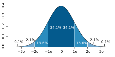
An example of how SE is used, is to make confidence intervals of the unknown population mean. If the sampling distribution is normally distributed, the sample mean, the standard error, and the quantiles of the normal distribution can be used to calculate confidence intervals for the true population mean. The following expressions can be used to calculate the upper and lower 95% confidence limits, where ${\bar {x}}$ is equal to the sample mean, $SE$ is equal to the standard error for the sample mean, and 1.96 is the 0.975 quantile of the normal distribution:

Upper 95% limit

={\bar {x}}+({\text{SE}}\times 1.96),

and

Lower 95% limit

={\bar {x}}-({\text{SE}}\times 1.96).

In particular, the standard error of a sample statistic (such as sample mean) is the actual or estimated standard deviation of the error in the process by which it was generated. In other words, it is the actual or estimated standard deviation of the sampling distribution of the sample statistic. The notation for standard error can be any one of SE, SEM (for standard error of measurement or mean), or S_E.

Standard errors provide simple measures of uncertainty in a value and are often used because:

in many cases, if the standard error of several individual quantities is known then the standard error of some function of the quantities can be easily calculated;
when the probability distribution of the value is known, it can be used to calculate an exact confidence interval;
when the probability distribution is unknown, Chebyshev's or the Vysochanskiï–Petunin inequalities can be used to calculate a conservative confidence interval; and
as the sample size tends to infinity the central limit theorem guarantees that the sampling distribution of the mean is asymptotically normal.

Standard error of mean versus standard deviation

In scientific and technical literature, experimental data are often summarized either using the mean and standard deviation of the sample data or the mean with the standard error. This often leads to confusion about their interchangeability. However, the mean and standard deviation are descriptive statistics, whereas the standard error of the mean is descriptive of the random sampling process. The standard deviation of the sample data is a description of the variation in measurements, while the standard error of the mean is a probabilistic statement about how the sample size will provide a better bound on estimates of the population mean, in light of the central limit theorem.^[5]

Put simply, the standard error of the sample mean is an estimate of how far the sample mean is likely to be from the population mean, whereas the standard deviation of the sample is the degree to which individuals within the sample differ from the sample mean. If the population standard deviation is finite, the standard error of the mean of the sample will tend to zero with increasing sample size, because the estimate of the population mean will improve, while the standard deviation of the sample will tend to approximate the population standard deviation as the sample size increases.

Correction for finite population

The formula given above for the standard error assumes that the sample size is much smaller than the population size, so that the population can be considered to be effectively infinite in size. This is usually the case even with finite populations, because most of the time, people are primarily interested in managing the processes that created the existing finite population; this is called an analytic study, following W. Edwards Deming. If people are interested in managing an existing finite population that will not change over time, then it is necessary to adjust for the population size; this is called an enumerative study.

When the sampling fraction is large (approximately at 5% or more) in an enumerative study, the estimate of the standard error must be corrected by multiplying by a "finite population correction":^[6] ^[7]

{\text{FPC}}={\sqrt {\frac {N-n}{N-1}}}

which, for large N:

{\text{FPC}}\approx {\sqrt {1-{\frac {n}{N}}}}

to account for the added precision gained by sampling close to a larger percentage of the population. The effect of the FPC is that the error becomes zero when the sample size n is equal to the population size N.

Correction for correlation in the sample

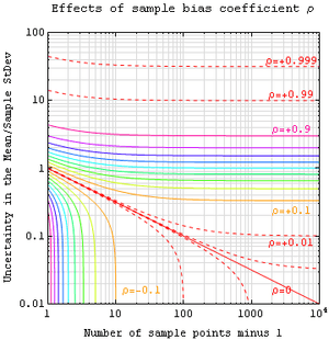
Expected error in the mean of A for a sample of n data points with sample bias coefficient ρ. The unbiased standard error plots as the ρ=0 diagonal line with log-log slope -½.

If values of the measured quantity A are not statistically independent but have been obtained from known locations in parameter space x, an unbiased estimate of the true standard error of the mean (actually a correction on the standard deviation part) may be obtained by multiplying the calculated standard error of the sample by the factor f:

f={\sqrt {\frac {1+\rho }{1-\rho }}},

where the sample bias coefficient ρ is the widely used Prais–Winsten estimate of the autocorrelation-coefficient (a quantity between −1 and +1) for all sample point pairs. This approximate formula is for moderate to large sample sizes; the reference gives the exact formulas for any sample size, and can be applied to heavily autocorrelated time series like Wall Street stock quotes. Moreover, this formula works for positive and negative ρ alike.^[8] See also unbiased estimation of standard deviation for more discussion.

Relative standard error

The relative standard error of a sample mean is the standard error divided by the mean and expressed as a percentage. It can only be calculated if the mean is a non-zero value.

As an example of the use of the relative standard error, consider two surveys of household income that both result in a sample mean of $50,000. If one survey has a standard error of $10,000 and the other has a standard error of $5,000, then the relative standard errors are 20% and 10% respectively. The survey with the lower relative standard error can be said to have a more precise measurement, since it has proportionately less sampling variation around the mean. In fact, data organizations often set reliability standards that their data must reach before publication. For example, the U.S. National Center for Health Statistics typically does not report an estimated mean if its relative standard error exceeds 30%. (NCHS also typically requires at least 30 observations – if not more – for an estimate to be reported.)^[9]

References

↑ Everitt, B. S. (2003). The Cambridge Dictionary of Statistics. CUP. ISBN 978-0-521-81099-9.
↑ Gurland, J; Tripathi RC (1971). "A simple approximation for unbiased estimation of the standard deviation". American Statistician. 25 (4): 30–32. doi:10.2307/2682923. JSTOR 2682923.
↑ Sokal; Rohlf (1981). Biometry: Principles and Practice of Statistics in Biological Research (2nd ed.). p. 53. ISBN 978-0-7167-1254-1.
↑ Hutchinson, T. P. Essentials of Statistical Methods, in 41 pages. Adelaide: Rumsby. ISBN 978-0-646-12621-0.
↑ Barde, M. (2012). "What to use to express the variability of data: Standard deviation or standard error of mean?". Perspect. Clin. Res. 3 (3): 113–116. doi:10.4103/2229-3485.100662. PMC 3487226. PMID 23125963.
↑ Isserlis, L. (1918). "On the value of a mean as calculated from a sample". Journal of the Royal Statistical Society. 81 (1): 75–81. doi:10.2307/2340569. JSTOR 2340569. (Equation 1)
↑ Bondy, Warren; Zlot, William (1976). "The Standard Error of the Mean and the Difference Between Means for Finite Populations". The American Statistician. 30 (2): 96–97. JSTOR 2683803. (Equation 2)
↑ Bence, James R. (1995). "Analysis of Short Time Series: Correcting for Autocorrelation". Ecology. 76 (2): 628–639. doi:10.2307/1941218. JSTOR 1941218.
↑ Klein, RJ. "Healthy People 2010 criteria for data suppression" (PDF). Statistical Notes (24). Retrieved 17 July 2014.

This article is issued from Wikipedia. The text is licensed under Creative Commons - Attribution - Sharealike. Additional terms may apply for the media files.

[1] Everitt, B. S. (2003). The Cambridge Dictionary of Statistics. CUP. ISBN 978-0-521-81099-9.

[2] Gurland, J; Tripathi RC (1971). "A simple approximation for unbiased estimation of the standard deviation". American Statistician. 25 (4): 30–32. doi:10.2307/2682923. JSTOR 2682923.

[3] Sokal; Rohlf (1981). Biometry: Principles and Practice of Statistics in Biological Research (2nd ed.). p. 53. ISBN 978-0-7167-1254-1.

[4] Hutchinson, T. P. Essentials of Statistical Methods, in 41 pages. Adelaide: Rumsby. ISBN 978-0-646-12621-0.

[5] Barde, M. (2012). "What to use to express the variability of data: Standard deviation or standard error of mean?". Perspect. Clin. Res. 3 (3): 113–116. doi:10.4103/2229-3485.100662. PMC 3487226. PMID 23125963.

[6] Isserlis, L. (1918). "On the value of a mean as calculated from a sample". Journal of the Royal Statistical Society. 81 (1): 75–81. doi:10.2307/2340569. JSTOR 2340569. (Equation 1)

[7] Bondy, Warren; Zlot, William (1976). "The Standard Error of the Mean and the Difference Between Means for Finite Populations". The American Statistician. 30 (2): 96–97. JSTOR 2683803. (Equation 2)

[8] Bence, James R. (1995). "Analysis of Short Time Series: Correcting for Autocorrelation". Ecology. 76 (2): 628–639. doi:10.2307/1941218. JSTOR 1941218.

[9] Klein, RJ. "Healthy People 2010 criteria for data suppression" (PDF). Statistical Notes (24). Retrieved 17 July 2014.