Discrete Global Grid

Geodesy
Fundamentals
Geodesy Geodynamics Geomatics Cartography History
Concepts
Geographical distance Geoid Figure of the Earth Geodetic datum Geodesic Geographic coordinate system Horizontal position representation Latitude / Longitude Map projection Reference ellipsoid Satellite geodesy Spatial reference system Spatial relations
Technologies
Global Nav. Sat. Systems (GNSSs) Global Pos. System (GPS) Galileo (Europe) GLONASS (Russia) BeiDou (BDS) (China) NAVIC (India) Quasi-Zenith Sat. Sys. (QZSS) (Japan) Discrete Global Grid and Geocoding
Standards (History)
NGVD 29 Sea Level Datum 1929 OSGB36 Ordnance Survey Great Britain 1936 SK-42 Systema Koordinat 1942 goda ED50 European Datum 1950 SAD69 South American Datum 1969 GRS 80 Geodetic Reference System 1980 ISO 6709 Geographic point coord. 1983 NAD 83 North American Datum 1983 WGS 84 World Geodetic System 1984 NAVD 88 N. American Vertical Datum 1988 ETRS89 European Terrestrial Ref. Sys. 1989 GCJ-02 Chinese obfuscated datum 2002 Geo URI Internet link to a point 2010 International Terrestrial Reference System Spatial Reference System Identifier (SRID) Universal Transverse Mercator (UTM)

A Discrete Global Grid (DGG) is a mosaic which covers the entire Earth's surface.

Mathematically it is a space partitioning: it consists of a set of non-empty regions that form a partition of the Earth’s surface.^[1] In an usual grid-modeling strategy, to simplify position calculations, each region is represented by a point, abstracting the grid as a set of region-points. Each region or region-point in the grid is called a cell.

When each cell of a grid is subject to a recursive partition, resulting in a "series of discrete global grids with progressively finer resolution"^[2], forming a hierarchical grid, it is named Hierarchical DGG (sometimes "DGG system").

Discrete Global Grids are used as the geometric basis for the building of geospatial data structures. Each cell is related with data objects or values, or (in the hierarchical case) may be associated with other cells. DGGs have been proposed for use in a wide range of geospatial applications, including vector and raster location representation, data fusion, and spatial databases.^[1]

The most usual grids are for horizontal position representation, using a standard datum, like WGS84. In this context is commom also to use a specific DGG as foundation for geocoding standardization.

In the context of a spatial index, a DGG can assign unique identifiers to each grid cell, using it for spatial indexing purposes, in geodatabases or for geocoding.

Reference model of the globe

The "globe", in the DGG concept, have no strict semantic; but in Geodesy a so-called "Grid Reference System" is a grid that divides space with precise positions relative to a datum, that is an approximated a "standard model of the Geoid". So, in the role of Geoid, the "globe" coverd by a DGG can be any of the following objects:

• The topographical surface of the Earth, when each cell of the grid have its surface-position coordinates and the elevantion in relation to the standard Geoid. Example: grid with coordinates (φ,λ,z) where z is the elevation.

• A standard Geoid surface. The z coordinate is zero for all grid, them can be omitted, (φ,λ).
  Ancient standards, before 1687 (the Newton's Principia publication), used a "reference sphere"; in nowadays the Geoid is mathematically abstracted as reference ellipsoid.
  • A simplified Geoid: sometimes an old geodesic standard (eg. SAD69) or a non-geodesic surface (e. g. perfectly spherical surface) must be adopted, and will covered by the grid. In this case cells must be labeled with non-ambiguous way, (φ',λ'), and the transformation (φ,λ)⟾(φ',λ') must be known.

• A projection surface. Typically the geographic coordinates (φ,λ) are projected (with some distortion) onto the 2D mapping plane with 2D Cartesian coordinates (x, y).

As a global modeling process, modern DGGs, when including projection process, tend to avoid surfaces like cylinder or a conic solids that result in discontinuities and indexing problems. Regular polyhedra and other topological equivalents of sphere led to the most promising known options to be covered by DGGs,^[1] because "spherical projections preserve the correct topology of the Earth – there are no singularities or discontinuities to deal with"^[3].

When working with a DGG it is important to specify which of these options was adopted. So, the characterization of the reference model of the globe of a DGG can be summarized by:

• The recovered object: the object type in the role of globe. If there are no projection, the object covered by the grid is the Geoid, the Earth or a sphere; else is the geometry class of the projection surface (e.g. a cylinder, a cube or a cone).

• Projection type: absent (no projection) or present. When present, its characterization can be summarized by the projection's goal property (e.g. equal-area, conformal, etc.) and the class of the corrective function (e.g. trigonometric, linear, quadractic, etc.).

NOTE: when the DGG is covering a projection surface, in a context of data provenance, the metadata about reference-Goid is also important — typical informing its ISO 19111's CRS value, with no confusion with the projection surface.

Types and examples

The main distinguishing feature to classify or compare DGGs is the use or not of an hierarchical grid structures:

• In hierarchical reference systems each cell is a "box reference" to a subset of cells, and cell identifiers can express this hierarchy in its numbering logic or structure.

• In non-hierarchical reference systems each cell have a distinc identifier and represents a fixed-scale region of the space. The discretization of the Latitude/Longitude system is the most popular, and the standard reference for conversions.

Other usual criteria to classify a DGG are tile-shape and granularity (grid resolution):

• Tile regularity and shape: there are regular, semi-regular or irregular grid. As in generic tilings by regular polygons, is possible to tiling with regular face (like wall tiles can be rectangular, triangular, hexagonal, etc.), or with same face type but changing its size or angles, resulting in semi-regular shapes.
  Uniformity of shape and regularity of metrics provide better grid-indexing algorithms. Although it has less practical use, totally irregular grids are possible, such in a Voronoi coverage.

• Fine or coarse granulation (cell size): modern DGGs are parametrizable in its grid resolution, so, it is a characteristic of the final DGG instance, but not usefull to classify DGGs, except when the DGG-type must use an specific resolution or have a discretization limit. A "fine" granulation grid is non-limited and "coarse" refers to drastic limitation. Historically the main limitations are related to digital/analogic media, the compression/expanded representations of the grid in a database, and the memory limitations to store the grid. When a quantitative characterization is necessary, the average area of the grid cells or average distance between cell centers can be adopted.

Non-hierarchical grids

The most common class of Discrete Global Grids are those that place cell center points on longitude/latitude meridians and parallels, or which use the longitude/latitude meridians and parallels to form the boundaries of rectangular cells. Examples of such grids, all based on Latitude/Longitude:

UTM zones Divides the Earth into sixty (strip) zones, each being a six-degree band of longitude. In digital media removes overlapping zone. Use secant transverse Mercator projection in each zone. Define 60 secant cylinders, 1 per zone. The UTM zones was enhanced by Military Grid Reference System (MGRS), by addiction of the Latitude bands.
inception: 1940s	coverd object: cylinder (60 options)	projection: UTM or latlong	irregular tiles: polygonal strips	grabularity: coarse

(modern) UTM - Universal Transverse Mercator Is a discretization of the continuous UTM grid, with a kind of 2-level hierarchy, where the first level (coarse grain) correspond to the "UTM zones with latitude bands" (the MGRS), use the same 60 cylinders as reference-projection objects. Each fine-grain cell is designated by an structured ID composed by "grid zone designator", "the 100,000-meter square identifier" and "numerical location". The grid resolution is a direct function of the number of digits in the coordinates, that is also standarized. For instance the cell 17N 630084 4833438 is a ~10mx10m square. PS: this standard use 60 distinct cylinders for projections. There are also "Regional Transverse Mercator" (RTM or UTM Regional) and "Local Transverse Mercator" (LTM or UTM Local) standards, with more specific cylinders, for better fit and precision at the point of interest.
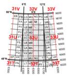inception: 1950s	coverd object: cylinder (60 options)	projection: UTM	rectangular tiles: equal-angle (conformal)	grabularity: fine

ISO 6709 Discretizes the traditional "graticule" representation and the modern numeric-coordinate cell-based locations. The granularity is fixed by a simple convention of the numeric representation, e. g. one-degree graticule, .01 degree graticule, etc. and it results in non-equal-area cells over the grid. The shape of the cells are rectangular except in the poles, where they are triangular. The numeric representation is standardized by two main conventions: degrees (Annex D) and decimal (Annex F). The grid resolution is controlled by the number of digits (Annex H).
inception: 1983	coverd object: Geoid (any ISO 19111's CRS)	projection: none	rectangular tiles: uniform spheroidal shape	grabularity: fine

Primary DEM (TIN DEM) A vector-based triangular irregular network (TIN) — the TIN DEM dataset is also referred to as a primary (measured) DEM. Many DEM are created on a grid of points placed at a regular angular increments of latitude and longitude. Examples include the Global 30 Arc-Second Elevation Dataset (GTOPO30).[4] and the Global Multi-resolution Terrain Elevation Data 2010 (GMTED2010) [5]. Triangulated irregular network is a representation of a continuous surface consisting entirely of triangular facets.
inception: 1970s	coverd object: terrain	projection: none	triangular non-uniform tiles: parametrized (vectorial)	grabularity: fine

Arakawa grids Was used for Earth system models for meteorology and oceanography — for example, the Global Environmental Multiscale Model (GEM) uses Arakawa grids for Global Climate Modeling.[6] The called "A-grid" the reference DGG, to be compared with other DGGs. Used in the 1980s with ~500x500 space resolutions.
inception: 1977	coverd object: geoid	projection: ?	rectangular tiles: parametric, space-time	grabularity: medium

WMO squares A specialiezed grid, used uniquely by NOAA, divides a chart of the world with latitude-longitude gridlines into grid cells of 10° latitude by 10° longitude, each with a unique, 4-digit numeric identifier (the first digit identifies quadrants NE/SE/SW/NW).
inception: 2001	coverd object: geoid	projection: none	Regular tiles: 36x18 rectangular cells	grabularity: coarse

World Grid Squares Are a compatible extension of Japanese Grid Squares standardized in Japan Industrial Standards (JIS X0410) to worldwide. The World Grid Square code can identify grid squares covering the world based on 6 layers. We can express a grid square by using from 6 to 13 digit sequence with accordance to its resolution.[7]
inception: ?	coverd object: geoid	projection: ?	? tiles: ?	grabularity: ?

Hierarchical grids

Successive space partitioning. The grey-and-green grid in the second and third maps are hierarchical.

The right aside illustration show 3 boundary maps of the coast of Great Britain. The first map was covered by a grid-level-0 with 150 km size cells. Only a grey cell in the center, with no need of zoom for detail, remains level-0; all other cells of the second map was partitioned into four-cells-grid (grid-level-1), each with 75 km. In the third map 12 cells level-1 remains as grey, all other was partitioned again, each level-1-cell transformed into a level-2-grid.
Examples of DGGs that use such recursive process, generating hierarchical grids, include:

ISEA Discrete Global Grids (ISEA DGGs) Are a class of grids proposed by researchers at Oregon State University.[1] The grid cells are created as regular polygons on the surface of an icosahedron, and then inversely projected using the Icosahedral Snyder Equal Area (ISEA) map projection[8] to form equal area cells on the sphere. Cells may be hexagons, triangles, or quadrilaterals. Multiple resolutions are indicated by choosing an aperture, or ratio between cell areas at consecutive resolutions. Some applications of ISEA DGGs include data products generated by the European Space Agency's Soil Moisture and Ocean Salinity (SMOS) satellite, which uses an ISEA4H9 (aperture 4 Hexagonal DGGS resolution 9),[9] and the commercial software Global Grid Systems Insight,[10] which uses an ISEA3H (aperture 3 Hexagonal DGGS).
inception: 1992..2004	coverd object: ?	projection: equal-area	parametrized (hexagons, triangles or quadrilaterals) tiles: equal-area	grabularity: fine

COBE - Quadrilateralized Spherical cube Cube[11]: Similar decomposition of sphere tham HEALPix and S2. But does not use space-filling curve, edges are not geodesics, and projection is more complicated.
inception: 1975..1991	coverd object: cube	projection: Curvilinear perspective	quadrilateral tiles: uniform area-preserving	grabularity: fine

Quaternary Triangular Mesh (QTM) QTM has triangular-shaped cells created by the 4-fold recursive subdivision of a spherical octahedron.[12]
inception: 1999 ... 2005	coverd object: octahedron (or other)	projection: Lambert's equal-area cylindrical	triangular tiles: uniform area-preserved	grabularity: fine

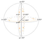
Hierarchical Equal Area isoLatitude Pixelization (HEALPix) HEALPix has equal area quadrilateral-shaped cells and was originally developed for use with full-sky astrophysical data sets.[13] The usual projecttion is "H=4, K=3 HEALPix projection". Main advantage, comparing with others of same indexing niche as S2, "is suitable for calculations involving spherical harmonics"[14].
inception: 2006	coverd object: Geoid	projection: (K,H) parametrized HEALPix projection	qradrilater tiles: uniform area-preserved	grabularity: fine

Hierarchical Triangular Mesh (HTM) Developed in 2003...2007, HTM "is a multi level, recursive decomposition of the sphere. It start with an octahedron, let this be level 0. As you project the edges of the octahedron onto the (unit) sphere creates 8 spherical triangles, 4 on the Northern and 4 on the Southern hemispheres".[15] The first public operational version seems[16] the HTM-v2 in 2004.
inception: 2004	coverd object: Geoid	projection: none	triangular tiles: spherical equilateres	grabularity: fine

Geohash Latitude and longitude are merged, enterlacing bits in the joined number. The binary result is represented with base32, offering a compact human-readable code. When used as spatial index, corresponds to a Z-order curve. There are some variants like Geohash-36.
inception: 2008	coverd object: Geoid	projection: none	semi-regular tiles: rectangular	grabularity: fine

S2 / S2Region The "S2 Grid System" is part of the "S2 Geometry Library"[17] (the name is derived from the mathematical notation for the n-sphere, S²). It implements an index system based on cube projection and the space-filling Hilbert curve, developed at Google.[18][19] The S2Region of S2 is the most general representation of its cells, where cell-position and metric (e.g. area) can be calculated. Each S2Region is a subgrid, resulting in a hierarchy limited to 31 levels. At level30 resolution is estimated[20] in 1 cm², at level0 is 85011012 km². The cell-identifier of the hierarchical grid of a cube face (6 faces) have and ID of 60 bits (so "every cm² on Earth can be represented using a 64-bit integer).
inception: 2015	coverd object: cube	projection: spherical projections in each cube face using quadratic function	semi-regular tiles: quadrilateral projections	grabularity: fine

S2 / S2LatLng The DGG supplied by S2LatLng representation, like an ISO 6709 grid, but hierarchical and with its specific cell shape.
inception: 2015	coverd object: Geoid or sphere	projection: none	semi-regular tiles: quadrilateral	grabularity: fine

S2 / S2CellId The DGG supplied by S2CellId representation. Each cell-ID is a 64-bit unsigned integer unique identifier, for any hierarchy level.
inception: 2015	coverd object: cube	projection: ?	semi-regular tiles: quadrilateral	grabularity: fine

Database modeling

In all DGG databases the grid is a composition of its cells. The region and centralPoint are illustrated as typical properties or subclasses. The cell identifier (cell ID) is also an important property, used as internal index and/or as public label of the cell (instead the point-coordinates) in geocoding applications. Sometimes, as in the MGRS grid, the coordinates make the role of ID.

There are many DGGs because there are many representational, optimization and modeling alternatives. All DGG grid is a composition of its cells, and, in the Hierarchical DGG each cell use a new grid over its local region.

The illustration is not adequate to TIN DEM cases and similar "raw data" structures, where the database not use the cell concept (that geometrically is the triangular region), but nodes and edges: each node is an elevation and each edge is the distance between to nodes.

In general each cell of the DGG is identified by the coordinates of its region-point (illustrated as the centralPoint of a database representation). It is also possible, with loss of functionality, to use a "free identifier", that is, any unique number or unique symbolic label per cell, the cell ID. The ID is usually used as spatial index (such as internal Quadtree or k-d tree), but is also possible to transform ID into a human-readable label for geocoding applications.

Modern databases (e.g. using S2 grid) use also multiple representations for the same data, offering both, a grid (or cell region) based in the Geoid and a grid based in the projection.

History

Discrete Global Grids with cell regions defined by parallels and meridians of latitude/longitude have been used since the earliest days of global geospatial computing. Before it, the discretization of continuous coordinates for practical purposes, with paper maps, occurred only with low granularity. Perhaps the most representative and main example of DGG of this pre-digital era was the 1940's military UTM DGGs, with finner granulaed cell identification for geocoding purposes. Similarly some hierarchical grid exists before geospatial computing, but only in coarse granulation.

A global surface is not required for use on daily geographical maps, and the memory was very expansive before the 2000s, to put all planetary data into the same computer. The first digital global grids was used for data processing of the satellite images and global (climatic and oceanographic) fluid dynamics modeling.

The first published references to Hierarchical Geodesic DGG systems are to systems developed for atmospheric modeling and published in 1968. These systems have hexagonal cell regions created on the surface of a spherical icosahedron. ^{[21] [22]}

The spatial hierarchical grids was subject to more intensive studies in the 1980's ^[23], when main structures, as Quadtree, was adapted in image indexing and databases.

While specific instances of these grids have been in use for decades, the term Discrete Global Grids were coined by researchers at Oregon State University in 1997^[2] to describe the class of all such entities.

Comparison and evolution

The evaluation Discrete Global Grid consists of many aspects, including area, shape, compactness, etc. Evaluation methods for map projection, such as Tissot's indicatrix, are also suitable for evaluating map projection based Discrete Global Grid.

The Hilbert curve adopted in DGGs like S2, for optimal spatial indexation. Was an evolution from Z-curve indexes, because have no "jumps", preserving nearest cells as neighbours.

In addition, averaged ratio between complementary profiles (AveRaComp) ^[24] gives a good evaluation of shape distortions for quadrilateral-shaped Discrete Global Grid.

Database development-choices and adaptations are oriented by practical demands, for greater performance, reliability or precision. The best choices are being selected and adapted to necessities, propitiating the evolution of the DGG architectures. Examples of this evolution process: from non-hierarchical to hierarchical DGGs; from the use of Z-curve indexes (a naive algorithm based in digits-interlacing), used by Geohash, to Hilbert-curve indexes, used in modern optimizations, like S2.

Geocoding variants

In general each cell of the grid is identified by the coordinates of its region-point, but it is also possible to simplify the coordinate syntax and semantics, to obtain a identifier, as in a classic alphanumeric grids — and find the coordinates of a region-point from its identifier. Small and fast coordinate representations is a goal in the cell-ID implementations, for any DGG solutions.

There are no loss of functionality when using a "free identifier" instead a coodinate, that is, any unique number or unique symbolic label per region-point, the cell ID. So, to transform a coordinate into a human-readable label, and/or compressing the length of the label, is an additional step in the grid repesentation.

Some popular "global place codes" as ISO 3166-1 alpha-2 for administrative regions or Longhurst code for ecological regions of the globe, are partial in globe's coverage. By other hand, any set of cell-identifiers of a specific DGG can be used as "full-coverage place codes". Each different set of IDs, when used as a standard for data interchange purposes, are named "geocoding system".

There are many ways to represent the value of a cell identifier (cell-ID) of a grid: structured or monolithic, binary or not, human-readable or not. Supposing a map feature, like the Singapore's Merlion fountaine (~5m scale feature), represented by its minimum bounding cell or a center-point-cell, the cell ID will be:

All these geocodes represents the same position in the globe, with similar precision, but differ in string-length, separators-use and alphabet (non-separator characters). In some cases the "original DGG" representation can be used. The variants are minor changes, affecting only final representation, for example the base of the numeric representation, or interlacing parts of the structured into only one number or code representation. The most popular variants are used for geocoding applications.

See also

• Grid reference
• Geodesic grid
• List of geocoding systems
• Military Grid Reference System

References

External links

• OGC DGGS Standards Working Group
• Discrete Global Grids page at the Computer Science department at Southern Oregon University
• BUGS climate model page on geodesic grids
• Research Institute for World Grid squares page on World Grid Squares

References

- 1 2 3 4 Sahr, Kevin; White, Denis; Kimerling, A.J. (2003). "Geodesic discrete global grid systems" (PDF). Cartography and Geographic Information Science. 30 (2): 121–134. doi:10.1559/152304003100011090.
- 1 2 Sahr, Kevin; White, Denis; Kimerling, A.J. (18 March 1997), "A Proposed Criteria for Evaluating Discrete Global Grids", Draft Technical Report, Corvallis, Oregon: Oregon State University
- ↑ http://s2geometry.io/about/overview
- ↑ "Global 30 Arc-Second Elevation (GTOPO30)". USGS. Retrieved October 8, 2015.
- ↑ "Global Multi-resolution Terrain Elevation Data 2010 (GMTED2010)". USGS. Retrieved October 8, 2015.
- ↑ Arakawa, A.; Lamb, V.R. (1977). "Computational design of the basic dynamical processes of the UCLA general circulation model". Methods of Computational Physics. 17. New York: Academic Press. pp. 173–265.
- ↑ "Research Institute for World Grid Squares". Kyoto University. Retrieved November 21, 2017.
- ↑ Snyder, J.P. (1992). "An equal-area map projection for polyhedral globes". Cartographica. 29 (1): 10–21. doi:10.3138/27h7-8k88-4882-1752.
- ↑ Suess, M.; Matos, P.; Gutierrez, A.; Zundo, M.; Martin-Neira, M. (2004). "Processing of SMOS level 1c data onto a discrete global grid". Proceedings of the IEEE International Geoscience and Remote Sensing Symposium: 1914–1917.
- ↑ "Global Grid Systems Insight". Global Grid Systems. Retrieved October 8, 2015.
- ↑ http://lambda.gsfc.nasa.gov/product/cobe/skymap_info_new.cfm
- ↑ Dutton, G. (1999). A hierarchical coordinate system for geoprocessing and cartography. Springer-Verlag.
- ↑ "HEALPix Background Purpose". NASA Jet Propulsion Laboratory. Retrieved October 8, 2015.
- ↑ https://s2geometry.io/devguide/s2cell_hierarchy
- ↑ http://skyserver.org/HTM
- ↑ http://www.adass.org/adass/proceedings/adass03/P3-9/
- ↑ http://s2geometry.io
- ↑ "Overview". s2geometry.io. Retrieved 2018-05-11.
- ↑ Kreiss, Sven (2016-07-27). "S2 cells and space-filling curves: Keys to building better digital map tools for cities". Medium. Retrieved 2018-05-11.
- ↑ http://s2geometry.io/resources/s2cell_statistics.html
- ↑ Sadourny, R.; Arakawa, A.; Mintz, Y. (1968). "Integration of the nondivergent barotropic vorticity equation with an icosahedral-hexagonal grid for the sphere". Monthly Weather Review. 96 (6): 351–356. doi:10.1175/1520-0493(1968)096<0351:iotnbv>2.0.co;2.
- ↑ Williamson, D.L. (1968). "Integration of the barotropic vorticity equation on a spherical geodesic grid". Tellus. 20 (4): 642–653. doi:10.1111/j.2153-3490.1968.tb00406.x.
- ↑ https://pdfs.semanticscholar.org/edaa/8fc5e196791c821a5c81e987e2f5ca3c6aa5.pdf
- ↑ Yan, Jin; Song, Xiao; Gong, Guanghong (2016). "Averaged ratio between complementary profiles for evaluating shape distortions of map projections and spherical hierarchical tessellations". Computers & Geosciences. 87: 41–55. doi:10.1016/j.cageo.2015.11.009. Retrieved 2015-11-27.
- ↑ "What3words: Find and share very precise locations via Google Maps with just 3 words". Retrieved 8 July 2014.
- ↑ https://github.com/google/open-location-code
- ↑ https://github.com/google/s2geometry