Intro
Boundary of Mandelbrot set consist of :[1]
- boundaries of primitive and satellite hyperbolic components of Mandelbrot set including points :
- Boundary of M without boundaries of hyperbolic components with points
- non-renormalizable (Misiurewicz with rational external angle and other).
- finitely renormalizable (Misiurewicz and other).
- infinitely renormalizble (Feigenbaum and other). Angle in turns of external rays landing on the Feigenbaum point are irrational numbers
- boundaries of non hyperbolic components ( we believe they do not exist but we cannot prove it ) Boundaries of non-hyperbolic components would be infinitely renormalizable as well.

Drawing boundaries
Methods used to draw boundary of Mandelbrot set :[2]
- whole boundary
- Distance Estimation Method for Mandelbrots set = DEM/M ( exterior, interior or both)
- Boundary scanning method (BSM) : detecting the edges after Boolean escape time [3]
- boundary tracing method [4][5]
- contour integration by Robert Davies[6]
- Jungreis function[7]
- implicit polynomial curves that converge to the boundary of the Mandelbrot set ( lemniscates)
- drawing boundaries of components of Mandelbrot set
How to draw whole M set boundary
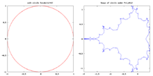
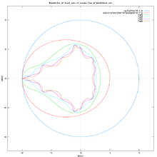
Jungreis function
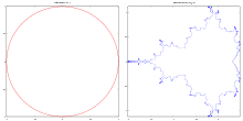
Description :
Python code
#!/usr/bin/env python
"""
    Python code by Matthias Meschede 2014
    http://pythology.blogspot.fr/2014/08/parametrized-mandelbrot-set-boundary-in.html
"""
import numpy as np
import matplotlib.pyplot as plt

nstore = 3000  #cachesize should be more or less as high as the coefficients
betaF_cachedata = np.zeros( (nstore,nstore))
betaF_cachemask = np.zeros( (nstore,nstore),dtype=bool)
def betaF(n,m):
    """
    This function was translated to python from
    http://fraktal.republika.pl/mset_jungreis.html
    It computes the Laurent series coefficients of the jungreis function
    that can then be used to map the unit circle to the Mandelbrot
    set boundary. The mapping of the unit circle can also
    be seen as a Fourier transform.
    I added a very simple global caching array to speed it up
    """
    global betaF_cachedata,betaF_cachemask

    nnn=2**(n+1)-1
    if betaF_cachemask[n,m]:
        return betaF_cachedata[n,m]
    elif m==0:
        return 1.0
    elif ((n>0) and (m < nnn)):
        return 0.0
    else:
        value = 0.
        for k in range(nnn,m-nnn+1):
            value += betaF(n,k)*betaF(n,m-k)
        value = (betaF(n+1,m) - value - betaF(0,m-nnn))/2.0
        betaF_cachedata[n,m] = value
        betaF_cachemask[n,m] = True
        return value

def main():
    #compute coefficients (reduce ncoeffs to make it faster)
    ncoeffs= 2400
    coeffs = np.zeros( (ncoeffs) )
    for m in range(ncoeffs):
        if m%100==0: print '%d/%d'%(m,ncoeffs)
        coeffs[m] = betaF(0,m+1)

    #map the unit circle  (cos(nt),sin(nt)) to the boundary
    npoints = 10000
    points = np.linspace(0,2*np.pi,npoints)
    xs     = np.zeros(npoints)
    ys     = np.zeros(npoints)
    xs = np.cos(points)
    ys = -np.sin(points)
    for ic,coeff in enumerate(coeffs):
        xs += coeff*np.cos(ic*points)
        ys += coeff*np.sin(ic*points)

    #plot the function
    plt.figure()
    plt.plot(xs,ys)
    plt.show()

if __name__ == "__main__":
    main()
How to draw boundaries of hyperbolic components
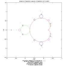
Methods of drawing boundaries:
- solving boundary equations :
- parametrisation of boundary with Newton method near centers of components[13] [14]. This methods needs centers, so it has some limitations,
- Boundary scanning : detecting the edges after detecting period by checking every pixel. This method is slow but allows zooming. Draws "all" components
- Boundary tracing for given c value. Draws single component.
- Fake Mandelbrot set by Anne M. Burns : draws main cardioid and all its descendants. Do not draw mini Mandelbrot sets. [15]
"... to draw the boundaries of hyperbolic components using Newton's method. That is, take a point in the hyperbolic component that you are interested in (where there is an attracting cycle), and then find a curve along which the modulus of the multiplier tends to one. Then you will have found an indifferent parameter. Now you can similarly change the argument of the multiplier, again using Newton's method, and trace this curve. Some care is required near "cusps". " Lasse Rempe-Gillen[16]
solving boundary equations
/*
c functions using complex type numbers
computes c from  component  of Mandelbrot set */
complex double Give_c( int Period,  int p, int q , double InternalRadius )
{

  complex double w;  // point of reference plane  where image of the component is a unit disk
  complex double c; // result
  double t; // InternalAngleInTurns

  t  = (double) p/q;
  t = t * M_PI * 2.0; // from turns to radians

  w = InternalRadius*cexp(I*t); // map to the unit disk

  switch ( Period ) // of component
    {
    case 1: // main cardioid = only one period 1 component
      c = w/2 - w*w/4; // https://en.wikibooks.org/wiki/Fractals/Iterations_in_the_complex_plane/Mandelbrot_set/boundary#Solving_system_of_equation_for_period_1
      break;
    case 2: // only one period 2 component
      c = (w-4)/4 ; // https://en.wikibooks.org/wiki/Fractals/Iterations_in_the_complex_plane/Mandelbrot_set/boundary#Solving_system_of_equation_for_period_2
      break;
      // period > 2
    default:
    	printf("higher periods : to do, use newton method \n");
    	printf("for each q = Period of the Child component  there are 2^(q-1) roots \n");
      	c = 0.0; //

      break; }
 return c;
}
System of 2 equations defining boundaries of period hyperbolic components

- first defines periodic point,
- second defines indifferent orbit ( multiplier of periodic point is equal to one ).

Because stability index is equal to radius of point of unit circle :


so one can change second equation to form [17] :

It gives system of equations :

It can be used for :
- drawing components ( boundaries, internal rays )
- finding indifferent parameters ( parabolic or for Siegel discs )
Above system of 2 equations has 3 variables : ( is constant and multiplier is a function of ). One have to remove 1 variable to be able to solve it.


Boundaries are closed curves : cardioids or circles. One can parametrize points of boundaries with angle ( here measured in turns from 0 to 1 ).

After evaluation of one can put it into above system, and get a system of 2 equations with 2 variables .

Now it can be solved
For periods:
- 1-3 it can be solved with symbolical methods and give implicit ( boundary equation) and explicit function (inverse multiplier map) :
- 1-2 it is easy to solve [18]
- 3 it can be solve using "elementary algebra" ( Stephenson )
- >3 it can't be reduced to explicitly function but
- can be reduced to implicit solution ( boundary equation) and solved numerically
- can be solved numerically using Newton method for solving system of nonlinear equations


Solving system of equation for period 1
Here is Maxima code :
(%i4) p:1;
(%o4) 1
(%i5) e1:F(p,z,c)=z;
(%o5) z^2+c=z
(%i6) e2:m(p)=w;
(%o6) 2*z=w
(%i8) s:eliminate ([e1,e2], [z]);
(%o8) [w^2-2*w+4*c]
(%i12) s:solve([s[1]], [c]);
(%o12) [c=-(w^2-2*w)/4]
(%i13) define (m1(w),rhs(s[1]));
(%o13) m1(w):=-(w^2-2*w)/4
where
w:exp(2*%pi*%i*t);
and
(%i15) display2d:false;
(%o15) false
(%i16) 2*w;
(%o16) 2*%e^(2*%i*%pi*t)
(%i17) w*w;
(%o17) %e^(4*%i*%pi*t)
Second equation contains only one variable, one can eliminate this variable. Because boundary equation is simple so it is easy to get explicit solution
m1(w):=-(w^2-2*w)/4
So
  m1(t) := block([w], w:exp(2*%pi*%i*t), return ((2*w-w^2)/4));
  g(t) := float(rectform(t));
Math equation:

Solving system of equation for period 2
Here is Maxima code using to_poly_solve package by Barton Willis:
(%i4) p:2;
(%o4) 2
(%i5) e1:F(p,z,c)=z;
(%o5) (z^2+c)^2+c=z
(%i6) e2:m(p)=w;
(%o6) 4*z*(z^2+c)=w
(%i7) e1:F(p,z,c)=z;
(%o7) (z^2+c)^2+c=z
(%i10) load(topoly_solver);
to_poly_solve([e1, e2], [z, c]);
(%o10) C:/PROGRA~1/MAXIMA~1.1/share/maxima/5.16.1/share/contrib/topoly_solver.mac
(%o11) [[z=sqrt(w)/2,c=-(w-2*sqrt(w))/4],[z=-sqrt(w)/2,c=-(w+2*sqrt(w))/4],[z=(sqrt(1-w)-1)/2,c=(w-4)/4],[z=-(sqrt(1-w)+1)/2,c=(w-4)/4]]
(%i12) s:to_poly_solve([e1, e2], [z, c]);
(%o12) [[z=sqrt(w)/2,c=-(w-2*sqrt(w))/4],[z=-sqrt(w)/2,c=-(w+2*sqrt(w))/4],[z=(sqrt(1-w)-1)/2,c=(w-4)/4],[z=-(sqrt(1-w)+1)/2,c=(w-4)/4]]
(%i14) rhs(s[4][2]);
(%o14) (w-4)/4
(%i16) define (m2 (w),rhs(s[4][2]));
(%o16) m2(w):=(w-4)/4
explicit solution :
m2(w):=(w-4)/4
Solving system of equation for period 3
For period 3 ( and higher) previous method give no results (Maxima code) :
(%i14) p:3;
e1:z=F(p,z,c);
e2:m(p)=w;
load(topoly_solver);
to_poly_solve([e1, e2], [z, c]);
(%o14) 3
(%o15) z=((z^2+c)^2+c)^2+c
(%o16) 8*z*(z^2+c)*((z^2+c)^2+c)=w
(%i17)
(%o17) C:/PROGRA~1/MAXIMA~1.1/share/maxima/5.16.1/share/contrib/topoly_solver.mac
`algsys' cannot solve - system too complicated.
#0: to_poly_solve(e=[z = ((z^2+c)^2+c)^2+c,8*z*(z^2+c)*((z^2+c)^2+c) = w],vars=[z,c])
-- an error.  To debug this try debugmode(true);
I use code by Robert P. Munafo[19] which is based on paper of Wolf Jung.
One can approximate period 3 components with equations [20] :
(%i1) z:x+y*%i;
(%o1)                              %i y + x
(%i2) w:asinh(z);
(%o2)                           asinh(%i y + x)
(%i3) realpart(w);
(%o3)
                                                         2    2
          2    2     2      2  2 1/4     atan2(2 x y, - y  + x  + 1)      2
log((((- y  + x  + 1)  + 4 x  y )    sin(---------------------------) + y)
                                                      2
                                                        2    2
         2    2     2      2  2 1/4     atan2(2 x y, - y  + x  + 1)      2
 + (((- y  + x  + 1)  + 4 x  y )    cos(---------------------------) + x) )/2
                                                     2
(%i4) imagpart(w);
                                                                2    2
                 2    2     2      2  2 1/4     atan2(2 x y, - y  + x  + 1)
(%o4) atan2(((- y  + x  + 1)  + 4 x  y )    sin(---------------------------)
                                                             2
                                                              2    2
               2    2     2      2  2 1/4     atan2(2 x y, - y  + x  + 1)
     + y, ((- y  + x  + 1)  + 4 x  y )    cos(---------------------------) + x)
Boundary equation
The result of solving above system with respect to is boundary equation,

where is boundary polynomial.

It defines exact coordinates of hyperbolic componenets for given period .

It is implicit equation.
Period 1
One can easly compute boundary point c

of period 1 hyperbolic component ( main cardioid) for given internal angle ( rotation number) t using this code by Wolf Jung[21]
t *= (2*PI); // from turns to radians
cx = 0.5*cos(t) - 0.25*cos(2*t);
cy = 0.5*sin(t) - 0.25*sin(2*t);
Period 2
t *= (2*PI);  // from turns to radians
cx = 0.25*cos(t) - 1.0;
cy = 0.25*sin(t);
Solving boundary equations
Solving boundary equations for various angles gives list of boundary points.
size
area of whole Mandelbrot set
size of the component
- estimated size of componnet
- on_the_precision_required_for_size_estimates by Claude Heiland-Allen
- deriving_the_size_estimate by Claude Heiland-Allen
- the N-2 rule[22]
- The approximation ( above ) was proved by Guckenheimer and McGehee : Guckenheimer, J., and McGehee, R., "a proof of the mandelbrot n2 conjecture," institut mittag-leffler, report 15, 1984.
- Bifurcation points and the "n-squared" approximation
- atom domain size
-- size-estimate.hs
-- http://www.fractalforums.com/mandelbrot-and-julia-set/some-questions-about-cardoids-circles-and-the-area/
import Data.Complex (Complex((:+)), polar)
import System.Environment (getArgs)

lambdabeta :: Int -> Complex Double -> (Complex Double, Complex Double)
lambdabeta period c = (lambda, beta)
  where
    zs = take period . iterate (\z -> z * z + c) $ 0
    lambdas = drop 1 . map (2 *) $ zs
    lambda = product lambdas
    beta = sum . map recip . scanl (*) 1 $ lambdas

sizeorient :: Int -> Complex Double -> (Double, Double)
sizeorient period c = polar . recip $ beta * lambda * lambda
  where
    (lambda, beta) = lambdabeta period c

main :: IO ()
main = do
  [p, x, y] <- getArgs
  let period = read p
      re     = read x
      im     = read y
      (size, orient) = sizeorient period (re :+ im)
  putStrLn $ "period = " ++ show period
  putStrLn $ "re     = " ++ show re
  putStrLn $ "im     = " ++ show im
  putStrLn $ "size   = " ++ show size
  putStrLn $ "orient = " ++ show orient
distinguish cardioids from pseudocircles
method of distinguish cardioids from pseudocircles is described in : Universal Mandelbrot Set by A. Dolotin. The relevant part is section 5, in particular equation 5.8. In the paper is defined implicitly in equation 5.1,


Equation 5.8 then becomes:

When epsilon is:
- near 0 then you have a cardioid
- near 1 then you have a circle
Code:
compute t from c
Function describing relation between parameter c and internal angle t :

It is used for computing c point of boundary of main cardioid
To compute t from c one can use Maxima CAS:
(%i1) eq1:c = exp(%pi*t*%i)/2 -  exp(2*%pi*t*%i)/4;


                               %i %pi t     2 %i %pi t
                             %e           %e
(%o1)                    c = ---------- - ------------
                                 2             4
(%i2) solve(eq1,t);
             %i log(1 - sqrt(1 - 4 c))        %i log(sqrt(1 - 4 c) + 1)
(%o2) [t = - -------------------------, t = - -------------------------]
                    %pi                              %pi
So :
 f1(c):=float(cabs( -  %i* log(1 - sqrt(1 - 4* c))/%pi));
 f2(c):=float(cabs( -  %i* log(1 + sqrt(1 - 4* c))/%pi));
References
- ↑ stackexchange : classification-of-points-in-the-mandelbrot-set
- ↑ mathoverflow : Parametrization of the boundary of the Mandelbrot set
- ↑ Boundary Scanning by Robert P. Munafo, 1993 Feb 3.
- ↑ The Almond Bread Homepage
- ↑ Efficient Boundary Tracking Through Sampling by Alex Chen , Todd Wittman , Alexander Tartakovsky , and Andrea Bertozzi
- ↑ http://www.robertnz.net/cx.htm contour integration by Robert Davies
- ↑ Jungreis function in wikipedia
- ↑ Drawing Mc by Jungreis Algorithm
- ↑ The Mandelbrot set approximated by the 4096 first Fourier coefficients of its boundary on twitter by gro_tsen :
- ↑ Image and Maxima CAS src code
- ↑ Mandelbrot set Components : image with descriptions and references
- ↑ Young Hee Geum, Kevin G. Hare : Groebner Basis, Resultants and the generalized Mandelbrot Set - methods for period 2 and higher, using factorization for finding irreducible polynomials
- ↑ Image : parametrisation of boundary with Newton method near centers of componentswith src code
- ↑ Mark McClure "Bifurcation sets and critical curves" - Mathematica in Education and Research, Volume 11, issue 1 (2006).
- ↑ Burns A M : Plotting the Escape: An Animation of Parabolic Bifurcations in the Mandelbrot Set. Mathematics Magazine, Vol. 75, No. 2 (Apr., 2002), pp. 104-116
- ↑ mathoverflow : what-are-good-methods-for-detecting-parabolic-components-and-siegel-disk-componen by Lasse Rempe-Gillen
- ↑ Newsgroups: gmane.comp.mathematics.maxima.general Subject: system of equations Date: 2008-08-11 21:44:39 GMT
- ↑ Thayer Watkins : The Structure of the Mandelbrot Set
- ↑ Brown Method by Robert P. Munafo
- ↑ A Parameterization of the Period 3 Hyperbolic Components of the Mandelbrot Set by Dante Giarrusso, Yuval Fisher
- ↑ Mandel: software for real and complex dynamics by Wolf Jung
- ↑ The Mandelbrot Set and Julia Sets Combinatorics in the Mandelbrot Set - The 1/n2 rule, and deviations from it