"Most programs for computing Julia sets work well when the underlying dynamics is hyperbolic but experience an exponential slowdown in the parabolic case." ( Mark Braverman )[1]
In other words it means that one can need days for making a good picture of parabolic Julia set with standard / naive algorithms.
There are 2 problems here :
- slow (= lazy) local dynamics ( in the neighbourhood of a parabolic fixed point )
- some parts are very thin ( hard to find using standard plane scanning)
Planes
Dynamic plane

Dynamic plane = complex z-plane :

- Julia set is a common boundary :
- Fatou set
- exterior of Julia set = basin of attraction to infinity :
- interior of Julia set = basin of attraction of finite, parabolic fixed point p :
- immediate basin = sum of componets which have parabolic fixed point p on it's boundary ; the immediate parabolic basin of p is the union of periodic connected components of the parabolic basin.


See also :
- Filled Julia set[3]

Key words
- parabolic chessboard or checkerboard
- parabolic implosion
- Fatou coordinate
- Hawaiian earring
- in wikipedia = "The plane figure formed by a sequence of circles that are all tangent to each other at the same point and such that the sequence of radii converges to zero." ( Barile, Margherita in MathWorld)[4]
- commons:Category:Hawaiian earrings
- Gevrey symptotic expansions
- the Écalle-Voronin invariants of (7.1) at the origin which have Gevrey- 1/2 asymptotic expansions[5]
- germ[6][7][8]
- germ of the function : Taylor expansion of the function
- multiplicity[9]
- Julia-Lavaurs sets
- The Leau-Fatou flower theorem:[10] repelling or attracting flower. Flower consist of petals
- Parabolic Linearization theorem
- The horn map
- Blaschke product
- Inou and Shishikura's near parabolic renormalization
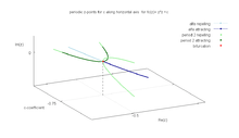
- complex polynomial vector field [11]
- numbers
- "a positive integer ν, the parabolic degeneracy with the following property: there are νq attracting petals and νq repelling petals, which alternate cyclically around the fixed point." [12]
- combinatorial rotation number
- a Poincaré linearizer of function f at parabolic fixed point[13]
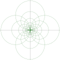
- " the parabolic pencil. This is the family of circles which all have one common point, and thus are all tangent to each other, either internally or externally. " [14]
Ecalle cilinder
Ecalle cylinders[15] or Ecalle-Voronin cylinders ( by Jean Ecalle[16][17])[18]
"... the quotient of a petal P under the equivalence relation identifying z and f (z) if both z and f (z) belong to P. This quotient manifold is called the Ecalle cilinder, and it is conformally isomorphic to the infinite cylinder C/Z"[19]
eggbeater dynamics
 Hand Egg beater
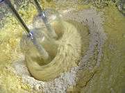 Here is real model of what happens in parabolic case
Physical model : the behaviour of cake when one uses eggbeater.
The mathematical model : a 2D vector field with 2 centers ( second-order degenerate points ) [20][21]
The field is spinning about the centers, but does not appear to be diverging.
Maybe better description of parabolic dynamics will be Hawaiian earrings
parabolic germ
- z+z^2
- z+z^3
- z+z^{k+1}
- z+a_{k+1}z^{k+1}
- z+a_{k+1}z^{k+1}
- "a germ with is holomorphically conjugated to its linear part " ( Sylvain Bonnot )[25]


germ of vector field
The horn map
" the horn map h = Φ ◦ Ψ, where Φ is a shorthand for Φattr and Ψ for Ψrep (extended Fatou coordinate and parameterizations)." [26]
Petal
_%3D_z%5E4_-_z_with_various_number_of_star_branches.gif)
"The petals ... are interesting not only because they give a rather good intuitive idea of the dynamics that arise near a parabolic point, but also because that the dynamic of f0 on a petal can be linearized, i.e., it is conjugated to the shift map T of C defined by T(w) := w + 1." ( Laurea Triennale [27] )
There is no unified definition of petals.
Petal of a flower can be :
- attracting / repelling
- small/alfa/big/ ( small attracting petals do not ovelap with repelling petals, but big do)
Each petal is invariant under f^period. In other words it is mapped to itself by f^period.
Attracting petal P is a :
- Each petal is invariant under . In other words it is mapped to itself by :
- domain (topological disc ) containing :
- parabolic periodic point p in its boundary ( precisely in its root , which is a coomon points of all attracting and repelling petals = center of the Lea-Fatou flower)
- critical point or it's n=period images on the other side ( only small ?? )
- trap which captures any orbit tending to parabolic point [28]
- set contained inside component of filled-in Julia set. The attracting petals of parabolic fixed point are contained in it's basin of attraction
- " ... is maximal with respect to this property. This preferred petal P max always has one or more critical points on its boundary."[29]
- "an attracting petal is the interior of an analytic curve which lies entirely in the Fatou set, has the right tangency property at the fixed point, and is mapped into its interior by the correct power of the map" Scott Sutherland
- "... an attracting petal is a set of points in a sufficient small disk around the periodic point whose forward orbits always remain in the disk under powers of return map. " ( W P Thurston : On the geometry and dynamics of Iterated rational maps)


Petals are symmetric with respect to the d-1 directions :


where :
- d is (to do)
- l is from 0 to d-2
Petals can have different size.
If then Julia set should approach parabolic periodic point in n directions, between n petals.[30]

" Using the language of holomorphic dynamics, people would say that you are studying the dynamics of a polynomial near the parabolic fixed point . By a simple linear change of variables, the study of any such parabolic fixed point can be reduced to the study of . Then you can apply another change . Thus you are reduced to the study of . If the real part $Re(w)$ is large enough you will obtain . This will give you what you want (when going back to the z-variable).


The domain (for large ) looks like some kind of cardioid (in your particular case) when you visualize it in the z-variable (it's poetically called an attracting petal). " Sylvain Bonnot [31]


Constructing the petal
0/1 or 1/1
 It is a dynamic plane for fc(z)=z^2 + 1/4. It is zoom around parabolic fixed point z=0.5. Orbits of some points inside Julia set are shown (white points)
_%3D_z%5E2_%2B0.25.svg.png) Attracting petals ( gray)
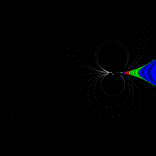
Attracting petals ( gray) Dynamics near parabolic fixed point
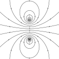 Contunuus model of dynamics inside a 1 petals flower ( dipol )
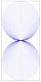
First attracting petal is a circle with:
- center on the x axis
- radius = ( cabs(zf) + cabs(z))/2
Other ( bigger ) attracting petals are preimages of first petal which include first petal
where:
- z is the last point of critical orbit
- zf is a fixed point
1/2
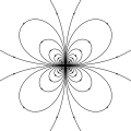 Model of dynamics inside a 2 petals flower (quadrupole)
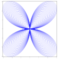
circular attracting petal:
- center is between fixed point and critical point
- radius smaller then half of the distance between fixed and critical point
// choose such value that level sets cross at z=0
// choose radius such a
double GivePetalRadius(complex double c, complex double fixed, int n){
	complex double z = 0.0; // critical point
	int k;
	// best for n>1
	int kMax = (n*ChildPeriod)  - 1; // ????

	for(k=0;  k<kMax-1; ++k)
		z = z*z + c; // forward iteration

	return  cabs(z-fixed)/2.0;


}
1/3
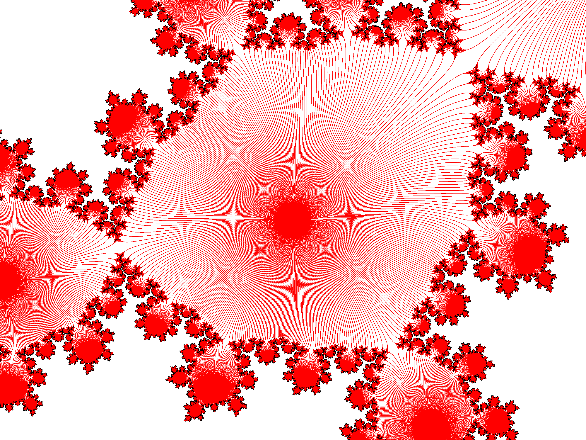
 Orbits near fixed point of fat Douady rabbit Julia set

Method by Scott Sutherland:[32]
- choose the connected component containing the critical point
- find an analytic curve which lies entirely in the Fatou set, has the right tangency property at the fixed point, and is mapped into its interior by the correct power of the map
- the other two are just the image of this curve under the first and second iterates.
Number of petals
For quadratic polynomials :
Multiplicity = ParentPeriod + ChildPeriod
NumberOfPetals = multiplicity - ParentPeriod
It is because in parabolic case fixed point coincidence with periodic cycle. Length of cycle ( child period) is equal to number of petals
For other polynomial maps :
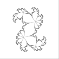
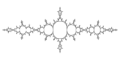
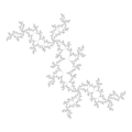
 One critical point and 5 petals
_%3D_z%5E14_-_z.png) 13 critical points and 26 petals.
13 critical points and 26 petals._%3D_z%5E15_-_z.png) 14 critical points and 14 petals.
14 critical points and 14 petals.%3Dz%5E4-z.png) z^4-z has 3 critical points and 6 petals
z^4-z has 3 critical points and 6 petals
| f(z) | number of petals | explanation |
|---|---|---|
| d-1 | for point z=0 has multiplicity d | |
| d+2 | (?)for a root z=0 has multiplicity d+3 | |


For f(z)= -z+z^(p+1) parabolic flower has :
- 2p petals for p odd
- p petals for p even [33]
... ( to do )
Sepal
_%3D_z%2Ba_2z_%5E2%2BO(z%5E3).png)

Definitions:
- A sepal is the intersection of an attracting and repelling petal.A parabolic Pommerenke-Levin-Yoccoz inequality. by Xavier Buf and Adam L. Epstein There does not seem to be an official definition of sepal.
- "Let l be an invariant curve in the first quadrant and L1 the region enclosed by l ∪ {0}, called a sepal." [34]
- interior of component with parabolic fixed point on it's boundary
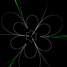
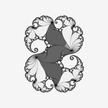
Flower
 Lea-Fatu flower
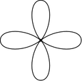 Flower with four petals and parabolic point in the center
- Critical orbit for internal angle 1/5 showing 5 attracting directions
Sum of all petals creates a flower with center at parabolic periodic point.[35]
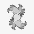
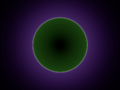
Cauliflower
Cauliflower or broccoli :[36]
- empty ( its interior is empty ) for c outside Mandelbrot set. Julia set is a totally disconnected (
- filled cauliflower for c=1/4 on boundary of the Mandelbrot set. Julia set is a Jordan curve ( quasi circle).
 c = 0 < 1/4
 c = 0.25 = 1/4 t he root of the main cardioid. Julia set is a cauliflower
 c = 0.255 > 1/4 "imploded cauliflower"
.jpg) c = 0.258 > 1/4
c = 0.258 > 1/4.jpg) c = [0.285, 0.01]
c = [0.285, 0.01]
Pleae note that :
- size of image differs because of different z-planes.
- different algorithms are used so colours are hard to compare
Bifurcation of the Cauliflower
How Julia set changes along real axis ( going from c=0 thru c=1/4 and further ) :
Perturbation of a function by complex :


When one add epsilon > 0 ( move along real axis toward + infinity ) there is a bifurcation of parabolic fixed point :
- attracting fixed point ( epsilon<0 )
- one parabolic fixed point ( epsilon = 0 )
- one parabolic fixed point splits up into two conjugate repelling fixed points ( epsilon > 0 )
"If we slightly perturb with epsilon<0 then the parabolic fixed point splits up into two real fixed points on the real axis (one attracting, one repelling). "
See :
- demo 2 page 9 in program Mandel by Wolf Jung
parabolic implosion
Video on YouTube[37]
Vector field
- 2D vector field and its
singularity
singularity types :
- center type : "In this case, one can find a neighborhood of the singular point where all integral curves are closed, inside one another, and contain the singular point in their interior" [38]
- non-center type : neighborhood of singularity is made of several curvilinear sectors :[39]
" A curvilinear sector is defined as the region bounded by a circle C with arbitrary small radius and two streamlines S and S! both converging towards singularity. One then considers the streamlines passing through the open sector g in order to distinguish between three possible types of curvilinear sectors."
Local dynamics
Local dynamics :
- in the exterior of Julia set
- on the Julia set
- near parabolic fixed point ( inside Julia set )
Near parabolic fixed point
Why analyze f^p not f ?
Forward orbit of f near parabolic fixed point is composite. It consist of 2 motions :
- around fixed point
- toward / away from fixed point
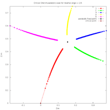
How to compute parabolic c values
| n | Internal angle (rotation number) t = 1/n | The root point c = parabolic parameter | Two external angles of parameter rays landing on the root point c (1/(2^n+1); 2/(2^n+1) | fixed point | external angles of dynamic rays landing on fixed point |
|---|---|---|---|---|---|
| 1 | 1/1 | 0.25 | (0/1 ; 1/1) | 0.5 | (0/1 = 1/1) |
| 2 | 1/2 | -0.75 | (1/3; 2/3) | -0.5 | (1/3; 2/3) |
| 3 | 1/3 | 0.64951905283833*%i-0.125 | (1/7; 2/7) | 0.43301270189222*%i-0.25 | (1/7; 2/7; 3/7) |
| 4 | 1/4 | 0.5*%i+0.25 | (1/15; 2/15) | 0.5*%i | (1/15; 2/15; 4/15; 8/15) |
| 5 | 1/5 | 0.32858194507446*%i+0.35676274578121 | (1/31; 2/31) | 0.47552825814758*%i+0.15450849718747 | (1/31; 2/31; 4/31; 8/31; 16/31) |
| 6 | 1/6 | 0.21650635094611*%i+0.375 | (1/63; 2/63) | 0.43301270189222*%i+0.25 | (1/63; 2/63; 4/63; 8/63; 16/63; 32/63) |
| 7 | 1/7 | 0.14718376318856*%i+0.36737513441845 | (1/127; 2/127) | 0.39091574123401*%i+0.31174490092937 | (1/127; 2/127, 4/127; 8/127; 16/127; 32/127, 64/127) |
| 8 | 1/8 | 0.10355339059327*%i+0.35355339059327 | 0.35355339059327*%i+0.35355339059327 | ||
| 9 | 1/9 | 0.075191866590218*%i+0.33961017714276 | 0.32139380484327*%i+0.38302222155949 | ||
| 10 | 1/10 | 0.056128497072448*%i+0.32725424859374 | 0.29389262614624*%i+0.40450849718747 |

For internal angle n/p parabolic period p cycle consist of one z-point with multiplicity p[40] and multiplier = 1.0 . This point z is equal to fixed point

Period 1
One can easily compute boundary point c

of period 1 hyperbolic component ( main cardioid) for given internal angle ( rotation number) t using this cpp code by Wolf Jung[41]
t *= (2*PI); // from turns to radians
cx = 0.5*cos(t) - 0.25*cos(2*t);
cy = 0.5*sin(t) - 0.25*sin(2*t);
or this Maxima CAS code :
/* conformal map  from circle to cardioid ( boundary
 of period 1 component of Mandelbrot set */
F(w):=w/2-w*w/4;

/*
circle D={w:abs(w)=1 } where w=l(t,r)
t is angle in turns ; 1 turn = 360 degree = 2*Pi radians
r is a radius
*/
ToCircle(t,r):=r*%e^(%i*t*2*%pi);

GiveC(angle,radius):=
(
 [w],
 /* point of  unit circle   w:l(internalAngle,internalRadius); */
 w:ToCircle(angle,radius),  /* point of circle */
 float(rectform(F(w)))    /* point on boundary of period 1 component of Mandelbrot set */
)$

compile(all)$

/* ---------- global constants & var ---------------------------*/
Numerator :1;
DenominatorMax :10;
InternalRadius:1;

/* --------- main -------------- */
for Denominator:1 thru DenominatorMax step 1 do
(
 InternalAngle: Numerator/Denominator,
 c: GiveC(InternalAngle,InternalRadius),
 display(Denominator),
 display(c),
  /* compute fixed point */
 alfa:float(rectform((1-sqrt(1-4*c))/2)), /* alfa fixed point */
 display(alfa)
 )$
Period 2
// cpp code by W Jung http://www.mndynamics.com
 t *= (2*PI);  // from turns to radians
 cx = 0.25*cos(t) - 1.0;
 cy = 0.25*sin(t);
Periods 1-6
/*

batch file for Maxima CAS
computing bifurcation points for period 1-6

 Formulae for cycles in the Mandelbrot set II
Stephenson, John; Ridgway, Douglas T.
Physica A, Volume 190, Issue 1-2, p. 104-116.
*/

kill(all);
remvalue(all);

start:elapsed_run_time ();

/* ------------ functions ----------------------*/

/* exponential for of complex number with angle in turns */
 /* "exponential form prevents allroots from working", code by Robert P. Munafo */

GivePoint(Radius,t):=rectform(ev(Radius*%e^(%i*t*2*%pi), numer))$ /* gives point of unit circle for angle t in turns */

GiveCirclePoint(t):=rectform(ev(%e^(%i*t*2*%pi), numer))$ /* gives point of unit circle for angle t in turns Radius = 1 */

/* gives a list of iMax points of unit circle */
GiveCirclePoints(iMax):=block(
 [circle_angles,CirclePoints],
 CirclePoints:[],
 circle_angles:makelist(i/iMax,i,0,iMax),
 for t in circle_angles do CirclePoints:cons(GivePoint(1,t),CirclePoints),
 return(CirclePoints) /* multipliers */
)$

/* http://commons.wikimedia.org/wiki/File:Mandelbrot_set_Components.jpg
Boundary equation  b_n(c,P)=0
    defines relations between hyperbolic components and unit circle for given period n ,
    allows computation of exact coordinates of hyperbolic componenets.

b_n(w,c), is boundary polynomial ( implicit function of 2 variables ).

*/

GiveBoundaryEq(P,n):=
block(
 if n=1 then return(c + P^2 - P),
 if n=2 then return(- c + P - 1),
 if n=3 then return(c^3 + 2*c^2 - (P-1)*c + (P-1)^2),
 if n=4 then return( c^6 + 3*c^5 + (P+3)* c^4 + (P+3)* c^3  - (P+2)*(P-1)*c^2 - (P-1)^3),
 if n=5 then return(c^15 + 8*c^14 + 28*c^13 + (P + 60)*c^12 + (7*P + 94)*c^11 +
  (3*P^2 + 20*P + 116)*c^10 + (11*P^2 + 33*P + 114)*c^9 + (6*P^2 + 40*P + 94)*c^8 +
  (2*P^3 - 20*P^2 + 37*P + 69)*c^7 + (3*P - 11)*(3*P^2 - 3*P - 4)*c^6 + (P - 1)*(3*P^3 + 20*P^2 - 33*P - 26)*c^5 +
  (3*P^2 + 27*P + 14)*(P - 1)^2*c^4 - (6*P + 5)*(P - 1)^3*c^3 + (P + 2)*(P - 1)^4*c^2 - c*(P - 1)^5  + (P - 1)^6),
if n=6 then return( c^27+
13*c^26+
78*c^25+
(293 - P)*c^24+
(792 - 10*P)*c^23+
(1672 - 41*P)*c^22+
(2892 - 84*P - 4*P^2)*c^21+
(4219 - 60*P - 30*P^2)*c^20+
(5313 + 155*P - 80*P^2)*c^19+
(5892 + 642*P - 57*P^2 + 4*P^3)*c^18+
(5843 + 1347*P + 195*P^2 + 22*P^3)*c^17+
(5258 + 2036*P + 734*P^2 + 22*P^3)*c^16+
(4346 + 2455*P + 1441*P^2 - 112*P^3 + 6*P^4)*c^15 +
(3310 + 2522*P + 1941*P^2 - 441*P^3 + 20*P^4)*c^14 +
(2331 + 2272*P + 1881*P^2 - 853*P^3 - 15*P^4)*c^13 +
(1525 + 1842*P + 1344*P^2 - 1157*P^3 - 124*P^4 - 6*P^5)*c^12 +
(927 + 1385*P + 570*P^2 - 1143*P^3 - 189*P^4 - 14*P^5)*c^11 +
(536 + 923*P - 126*P^2 - 774*P^3 - 186*P^4 + 11*P^5)*c^10 +
(298 + 834*P + 367*P^2 + 45*P^3 - 4*P^4 + 4*P^5)*(1-P)*c^9 +
(155 + 445*P - 148*P^2 - 109*P^3 + 103*P^4 + 2*P^5)*(1-P)*c^8 +
2*(38 + 142*P - 37*P^2 - 62*P^3 + 17*P^4)*(1-P)^2*c^7 +
(35 + 166*P + 18*P^2 - 75*P^3 - 4*P^4)*((1-P)^3)*c^6 +
(17 + 94*P + 62*P^2 + 2*P^3)*((1-P)^4)*c^5 +
(7 + 34*P + 8*P^2)*((1-P)^5)*c^4 +
(3 + 10*P + P^2)*((1-P)^6)*c^3 +
(1 + P)*((1-P)^7)*c^2 +
-c*((1-P)^8) + (1-P)^9)
)$

/* gives a list of points c on boundaries on all components for give period */
GiveBoundaryPoints(period,Circle_Points):=block(
 [Boundary,P,eq,roots],
  Boundary:[],
 for m in Circle_Points do (/* map from reference plane to parameter plane */
  P:m/2^period,
  eq:GiveBoundaryEq(P,period), /* Boundary equation  b_n(c,P)=0  */
  roots:bfallroots(%i*eq),
  roots:map(rhs,roots),
  for root in roots do Boundary:cons(root,Boundary)),
  return(Boundary)
)$

/* divide llist of roots to 3 sublists = 3  components */
/* ---- boundaries of period 3 components
period:3$
Boundary3Left:[]$
Boundary3Up:[]$
Boundary3Down:[]$

Radius:1;

 for m in CirclePoints do (
  P:m/2^period,
  eq:GiveBoundaryEq(P,period),
  roots:bfallroots(%i*eq),
  roots:map(rhs,roots),
  for root in roots do
     (
       if realpart(root)<-1  then Boundary3Left:cons(root,Boundary3Left),
       if (realpart(root)>-1 and imagpart(root)>0.5)
            then Boundary3Up:cons(root,Boundary3Up),
       if (realpart(root)>-1 and imagpart(root)<0.5)
            then Boundary3Down:cons(root,Boundary3Down)

     )

)$
--------- */

/* gives a list of parabolic points for given : period and internal angle */
GiveParabolicPoints(period,t):=block
(
 [m,ParabolicPoints,P,eq,roots],
 m: GiveCirclePoint(t), /* root of unit circle, Radius=1, angle t=0 */
 ParabolicPoints:[],
 /* map from reference plane to parameter plane */
 P:m/2^period,
 eq:GiveBoundaryEq(P,period), /* Boundary equation  b_n(c,P)=0  */
 roots:bfallroots(%i*eq),
 roots:map(rhs,roots),
 for root in roots do ParabolicPoints:cons(float(root),ParabolicPoints),
 return(ParabolicPoints)

)$

compile(all)$

/* ------------- constant values ----------------------*/

fpprec:16;

/* ------------unit circle on a w-plane -----------------------------------------*/
a:GiveParabolicPoints(6,1/3);
a$
How to draw parabolic Julia set
- 5 methods of drawing
 Checking iteration
 modified DEM
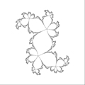 checking angle
 checking if zn is in target set
 checking if zn is in triangle target set
All points of interior of filled Julia set tend to one periodic orbit ( or fixed point ). This point is in Julia set and is weakly attracting.[42] One can analyse only behevior near parabolic fixed point. It can be done using critical orbits.
There are two cases here : easy and hard.
If the Julia set near parabolic fixed point is like n-th arm star ( not twisted) then one can simply check argument of of zn, relative to the fixed point. See for example z+z^5. This is an easy case.
In the hard case Julia set is twisted around fixed.
Estimation from exterior
Escape time
Long iteration method
Long iteration method [43]
Dynamic rays
One can use periodic dynamic rays landing on parabolic fixed point to find narrow parts of exterior.
Let's check how many backward iterations needs point on periodic ray with external radius = 4 to reach distance 0.003 from parabolic fixed point :
| period | Inverse iterations | time |
|---|---|---|
| 1 | 340 | 0m0.021s |
| 2 | 55 573 | 0m5.517s |
| 3 | 8 084 815 | 13m13.800s |
| 4 | 1 059 839 105 | 1724m28.990s |
| C source code - click on the right to view |
|---|
| a.c: |
/*
c console program
to compile  :
 gcc double_t.c -lm -Wall -march=native

to run :
time ./a.out

period	EscapeTime	time
1	       340	 0m0.021s
2	    55 573   	 0m5.517s
3	 8 084 815	13m13.800s
4    1 059 839 105    1724m28.990s

period 1
escape time   = 340.000000
internal angle t  = 1.000000
period  = 1
preperiod  = 0
cx  = 0.250000
cy  = 0.000000
alfax  = 0.500000
alfay  = 0.000000
real	0m0.021s

===============
escape time   = 55573.000000
internal angle t  = 0.500000
period  = 2
preperiod  = 0
cx  = -0.750000
cy  = 0.000000
alfax  = -0.500000
alfay  = 0.000000

real	0m5.517s
===============================
period = 3  c = (-0.125000; 0.649519); alfa  = (-0.250000;0.433013)
ea  = 0.142857;
internal angle t  = 0.333333
preperiod  = 0
for period = 3  escape time =    8084815

real	13m13.800s
=====================================
period = 4  c = (0.250000; 0.500000); alfa  = (0.000000;0.500000)
ea  = 0.066667;
internal angle t  = 0.250000
preperiod  = 0
for period = 4  escape time = 1059839105

real	1724m28.990s

*/

#include <stdio.h>
#include <stdlib.h> // malloc
#include <math.h> // M_PI; needs -lm also
#include <complex.h>

unsigned int period = 4;// of child component of Mandelbrot set
unsigned int numerator=1 ;
unsigned int denominator;
double t ; // internal angle of point c of parent component of Mandelbrot set in turns
unsigned long int maxiter = 100000;
unsigned int preperiod = 0; //of external angle under doubling map

 double complex z , c, alfa;
  double ea ;// External Angle

/* find c in component of Mandelbrot set
 uses complex type so #include <complex.h> and -lm
 uses code by Wolf Jung from program Mandel
 see function mndlbrot::bifurcate from mandelbrot.cpp
 http://www.mndynamics.com/indexp.html

  */
double complex GiveC(double InternalAngleInTurns, double InternalRadius, unsigned int period)
{
  //0 <= InternalRay<= 1
  //0 <= InternalAngleInTurns <=1
  // period of parent component of Mandelbrot set  { 1,2 }
  double t = InternalAngleInTurns *2*M_PI; // from turns to radians
  double R2 = InternalRadius * InternalRadius;
  double Cx, Cy; /* C = Cx+Cy*i */
  switch ( period ) {
    case 1: // main cardioid
      Cx = (cos(t)*InternalRadius)/2-(cos(2*t)*R2)/4;
      Cy = (sin(t)*InternalRadius)/2-(sin(2*t)*R2)/4;
      break;
   case 2: // only one component
      Cx = InternalRadius * 0.25*cos(t) - 1.0;
      Cy = InternalRadius * 0.25*sin(t);
      break;
  // for each period  there are 2^(period-1) roots.
  default: // safe values
      Cx = 0.0;
      Cy = 0.0;
    break; }

  return Cx+ Cy*I;
}

/*

http://en.wikipedia.org/wiki/Periodic_points_of_complex_quadratic_mappings
z^2 + c = z
z^2 - z + c = 0
ax^2 +bx + c =0 // ge3neral for  of quadratic equation
so :
a=1
b =-1
c = c
so :

The discriminant is the  d=b^2- 4ac

d=1-4c = dx+dy*i
r(d)=sqrt(dx^2 + dy^2)
sqrt(d) = sqrt((r+dx)/2)+-sqrt((r-dx)/2)*i = sx +- sy*i

x1=(1+sqrt(d))/2 = beta = (1+sx+sy*i)/2

x2=(1-sqrt(d))/2 = alfa = (1-sx -sy*i)/2

alfa : attracting when c is in main cardioid of Mandelbrot set, then it is in interior of Filled-in Julia set, it means belongs to Fatou set ( strictly to basin of attraction of finite fixed point )
*/
// uses global variables :
//  ax, ay (output = alfa(c))
double complex GiveAlfaFixedPoint(double complex c)
{
  double dx, dy; //The discriminant is the  d=b^2- 4ac = dx+dy*i
  double r; // r(d)=sqrt(dx^2 + dy^2)
  double sx, sy; // s = sqrt(d) = sqrt((r+dx)/2)+-sqrt((r-dx)/2)*i = sx + sy*i
  double ax, ay;

 // d=1-4c = dx+dy*i
 dx = 1 - 4*creal(c);
 dy = -4 * cimag(c);
 // r(d)=sqrt(dx^2 + dy^2)
 r = sqrt(dx*dx + dy*dy);
 //sqrt(d) = s =sx +sy*i
 sx = sqrt((r+dx)/2);
 sy = sqrt((r-dx)/2);
 // alfa = ax +ay*i = (1-sqrt(d))/2 = (1-sx + sy*i)/2
 ax = 0.5 - sx/2.0;
 ay =  sy/2.0;

return ax+ay*I;
}

double DistanceBetween(double complex z1, double complex z2 )
{double dx,dy;

 dx = creal(z1) - creal(z2);
 dy = cimag(z1) - cimag(z2);
 return sqrt(dx*dx+dy*dy);

}

/*
 principal square  root of complex number
 http://en.wikipedia.org/wiki/Square_root

 z1= I;
  z2 = root(z1);
  printf("zx  = %f \n", creal(z2));
  printf("zy  = %f \n", cimag(z2));
*/
double complex root(double complex z)
{
  double x = creal(z);
  double y = cimag(z);
  double u;
  double v;
  double r = sqrt(x*x + y*y);

  v = sqrt(0.5*(r - x));
  if (y < 0) v = -v;
  u = sqrt(0.5*(r + x));
 return u + v*I;
}

double complex preimage(double complex z1, double complex z2,  double complex c)
{
  double complex zPrev;

  zPrev = root(creal(z1) - creal(c) + ( cimag(z1) - cimag(c))*I);
  // choose one of 2 roots
  if (creal(zPrev)*creal(z2) + cimag(zPrev)*cimag(z2) > 0)
        return zPrev ;     //  u+v*i
       else return -zPrev; // -u-v*i
}

// This function only works for periodic or preperiodic angles.
// You must determine the period n and the preperiod k before calling this function.
// based on same function from src code of program Mandel by Wolf Jung
// http://www.mndynamics.com/indexp.html
double  backray(double t, // external angle in turns
		       int n, //period of ray's angle under doubling map
		       int k, // preperiod
                       int iterMax,
                       double complex c
                          )
{
  double xend ; // re of the endpoint of the ray
  double yend; // im of the endpoint of the ray
  const double R = 4; // very big radius = near infinity
  int j; // number of ray
  double iter=0.0; // index of backward iteration


  double complex zPrev;
  double u,v; // zPrev = u+v*I
  double complex zNext;
  double distance;

   /* dynamic 1D arrays for coordinates ( x, y) of points with the same R on preperiodic and periodic rays  */
  double *RayXs, *RayYs;
  int iLength = n+k+2; // length of arrays ?? why +2
  //  creates arrays :  RayXs and RayYs  and checks if it was done
  RayXs = malloc( iLength * sizeof(double) );
  RayYs = malloc( iLength * sizeof(double) );
  if (RayXs == NULL || RayYs==NULL)
    {
      fprintf(stderr,"Could not allocate memory");
      getchar();
      return 1;
    }

 //  starting points on preperiodic and periodic rays
 //  with angles t, 2t, 4t...  and the same radius R
  for (j = 0; j < n + k; j++)
  { // z= R*exp(2*Pi*t)
    RayXs[j] = R*cos((2*M_PI)*t);
    RayYs[j] = R*sin((2*M_PI)*t);
    t *= 2; // t = 2*t
    if (t > 1) t--; // t = t modulo 1
  }
  zNext = RayXs[0] + RayYs[0] *I;

  //printf("RayXs[0]  = %f \n", RayXs[0]);
  //printf("RayYs[0]  = %f \n", RayYs[0]);

  // z[k] is n-periodic. So it can be defined here explicitly as well.
  RayXs[n+k] = RayXs[k];
  RayYs[n+k] = RayYs[k];

  //   backward iteration of each point z
  do
    {

        for (j = 0; j < n+k; j++) // period +preperiod
         { // u+v*i = sqrt(z-c)   backward iteration in fc plane
		zPrev = root(RayXs[j+1] - creal(c)+(RayYs[j+1] - cimag(c))*I ); // , u, v
                u=creal(zPrev);
                v=cimag(zPrev);

		// choose one of 2 roots: u+v*i or -u-v*i
		if (u*RayXs[j] + v*RayYs[j] > 0)
                        { RayXs[j] = u; RayYs[j] = v; } // u+v*i
			else { RayXs[j] = -u; RayYs[j] = -v; } // -u-v*i
         } // for j ...

          //RayYs[n+k] cannot be constructed as a preimage of RayYs[n+k+1]
          RayXs[n+k] = RayXs[k];
          RayYs[n+k] = RayYs[k];

          // convert to pixel coordinates
          //  if z  is in window then draw a line from (I,K) to (u,v) = part of ray

       // printf("for iter = %d cabs(z) = %f \n", iter, cabs(RayXs[0] + RayYs[0]*I));
   iter += 1.0;
  distance = DistanceBetween(RayXs[j]+RayYs[j]*I, alfa);
   printf("distance  = %10.9f ; iter = %10.0f \n", distance, iter); // info
  }
 while (distance>0.003);// distance < pixel size

 // last point of a ray 0
 xend = RayXs[0];
 yend = RayYs[0];

 // free memmory
 free(RayXs);
 free(RayYs);

return  iter; //
}

/* ---------------------- main ------------------*/
int main()
{

 double EscapeTime;

  // internal angle
  denominator = period;
  t = (double) numerator/denominator;

  //
  c = GiveC(t, 1.0, 1);
  alfa = GiveAlfaFixedPoint(c);

  //external angle
  denominator= pow(2,period) - 1;
  ea = (double) 1.0/ denominator;
  //
  EscapeTime = backray(ea, period, preperiod, maxiter, c );


  //
  printf("period = %d ", period );
  printf(" c = (%f; %f);", creal(c), cimag(c));
  printf(" alfa  = (%f;%f)\n", creal(alfa), cimag(alfa));
  printf("ea  = %f;\n", ea);
  printf("internal angle t  = %f \n", t);
  printf("preperiod  = %d \n", preperiod);
  printf("for period = %d  escape time = %10.0f \n", period,  EscapeTime);
  //


  return 0;
}
|
One can use only argument of point z of external rays and its distance to alfa fixed point. ( see code from image) It works for periods up to 15 ( maybe more ... )
Estimation from interior
Julia set is a boundary of filled-in Julia set Kc.
- find points of interior of Kc
- find boundary of interior of Kc using edge detection
If components of interior are lying very close to each other then find components using :[44]
color = LastIteration % period
For parabolic components between parent and child component :[45]
periodOfChild = denominator*periodOfParent
color = iLastIteration % periodOfChild
where denominator is a denominator of internal angle of parent comonent of Mandelbrot set.
Angle
"if the iterate zn of tends to a fixed parabolic point, then the initial seed z0 is classified according to the argument of zn−z0, the classification being provided by the flower theorem " ( Mark McClure [46])
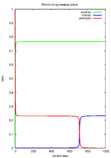
Attraction time
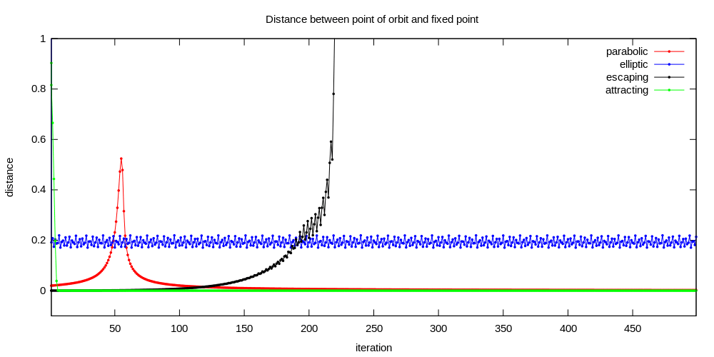
Interior of filled Julia set consist of components. All comonents are preperiodic, some of them are periodic ( immediate basin of attraction).
In other words :
- one iteration moves z to another component ( and whole component to another component)
- all point of components have the same attraction time ( number of iteration needed to reach target set around attractor)
It is possible to use it to color components. Because in parabolic case attractor is weak ( weakly attracting) it needs a lot of iterations for some points to reach it.
 // i = number of iteration
 // iPeriodChild = period of child component of Mandelbrot set ( parabolic c value is a root point between parant and child component
 /* distance from z to Alpha  */
 Zxt=Zx-dAlfaX;
 Zyt=Zy-dAlfaY;
 d2=Zxt*Zxt +Zyt*Zyt;
 // interior : check if fall into internal target set ( circle around alfa fixed point )
 if (d2<dMaxDistance2Alfa2) return  iColorsOfInterior[i % iPeriodChild];
Here are some example values :
 iWidth  = 1001 // width of image in pixels
 PixelWidth  = 0.003996
 AR  = 0.003996 // Radius around attractor
 denominator  = 1 ; Cx  = 0.250000000000000; Cy  = 0.000000000000000 ax  = 0.500000000000000; ay  = 0.000000000000000
 denominator  = 2 ; Cx  = -0.750000000000000; Cy  = 0.000000000000000 ax  = -0.500000000000000; ay  = 0.000000000000000
 denominator  = 3 ; Cx  = -0.125000000000000; Cy  = 0.649519052838329 ax  = -0.250000000000000; ay  = 0.433012701892219
 denominator  = 4 ; Cx  = 0.250000000000000; Cy  = 0.500000000000000 ax  = 0.000000000000000; ay  = 0.500000000000000
 denominator  = 5 ; Cx  = 0.356762745781211; Cy  = 0.328581945074458 ax  = 0.154508497187474; ay  = 0.475528258147577
 denominator  = 6 ; Cx  = 0.375000000000000; Cy  = 0.216506350946110 ax  = 0.250000000000000; ay  = 0.433012701892219

 denominator  = 1 ;   i =               243.000000
 denominator  = 2 ;   i =            31 171.000000
 denominator  = 3 ;   i =         3 400 099.000000
 denominator  = 4 ;   i =       333 293 206.000000
 denominator  = 5 ;   i =    29 519 565 177.000000
 denominator  = 6 ;   i = 2 384 557 783 634.000000
where :
C = Cx + Cy*i
a = ax + ay*i // fixed point alpha
i // number of iterations after which critical point z=0.0 reaches disc around fixed point alpha with radius AR
denominator of internal angle ( in turns )
internal angle =  1/denominator
Note that attraction time i is proportional to denominator.
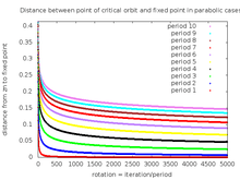
Now you see what means weakly attracting.
One can :
- use brutal force method ( Attracting radius < pixelSize; iteration Max big enough to let all points from interior reach target set; long time or fast computer )
- find better method (:-)) if time is to long for you
Interior distance estimation
Trap
Estimation from interior and exterior
Julia set is a common boundary of filled-in Julia set and basin of attraction of infinity.
- find points of interior/components of Kc
- find escaping points
- find boundary points using Sobel filter
It works for denominator up to 4.
Inverse iteration of repelling points
Inverse iteration of alfa fixed point. It works good only for cuting point ( where external rays land). Other points still are not hitten.
Bof61
Gallery
- Critical orbits in case of one critical point
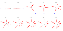 critical orbits for internal angle from 1/1 to 1/10. True attracting directions
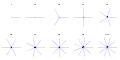 N-th arm stars for n from 1 to 10. Schematic attracting directions
%3Dz%5E2_%2B_mz_where_p_over_q%3D1_over_3.svg.png) critical orbit, attracting and repelling vectors for internal angle 1/3
critical orbit, attracting and repelling vectors for internal angle 1/3
- from period 1 thru ...
- 1/1 cauliflower
 1/2 San Marco fractal [47]
 1/3 Douady fat rabbit [48]
- 1/4
- 1/5
 1/7
1/7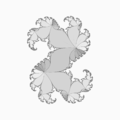 1/10
1/10- 1/15
- 1/20
- 1/30
- from period 2 thru ...
- from 2 thru internal ray 1/1 ; c=-0.75 Julia set is a San Marco fractal [49]
 from period 2 thru 1/2
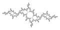 from period 2 thru 1/3
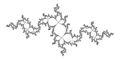 from period 2 thru 1/4
- from period 3 thru ...
 from period 3 thru 1/3
External examples:
See also
- Image : Nonstandard Parabolic by Cheritat[50]
- Julia set of parabolic case in Maxima CAS[51]
- The parabolic Mandelbrot set Pascale ROESCH (joint work with C. L. PETERSEN
- PARABOLIC IMPLOSION A MINI-COURSE by ArnaudCheritat
- Workshop on parabolic implosion 2010
- The renormalization for parabolic fixed points... Mitsushiro Shishikura and Hiroyuki Inou
- Dynamics of holomorphic maps: Resurgence of Fatou coordinates, and Poly-time computability of Julia sets by Artem Dudko, arxiv.org : Dudko_A
- Minicourse "Analytic classification of germs of generic families unfolding a parabolic point by Christiane Rousseau
- Perspectives on Parabolic Points in Holomorphic Dynamics - The Banff International Research Station for Mathematical Innovation and Discovery (BIRS)
- Richard Oudkerk : The Parabolic Implosion for f_0(z) = z + z^{nu+1} + O(z^{nu+2})
- Perspectives on Parabolic Points in Holomorphic Dynamics Videos from BIRS Workshop 15w5082
- Generic Perturbation of Parabolic Points Having More Than One Attracting Petal by Arnaud Chéritat
References
- ↑ Mark Braverman : On efficient computation of parabolic Julia sets
- ↑ Note on dynamically stable perturbations of parabolics by Tomoki Kawahira
- ↑ Filled Julia set in wikipedia
- ↑ Barile, Margherita. "Hawaiian Earring." From MathWorld--A Wolfram Web Resource, created by Eric W. Weisstein. http://mathworld.wolfram.com/HawaiianEarring.html
- ↑ Augustin Fruchard, Reinhard Sch¨afke. Composite Asymptotic Expansions and Difference Equations. Revue Africaine de la Recherche en Informatique et Math´ematiques Appliqu´ees, INRIA, 2015, 20, pp.63-93. <hal-01320625>
- ↑ wikipedia : Germ(mathematics)
- ↑ Fixed points of diffeomorphisms, singularities of vector fields and epsilon-neighborhoods of their orbits by Maja Resman
- ↑ The moduli space of germs of generic families of analytic diffeomorphisms unfolding a parabolic fixed point by Colin Christopher, Christiane Rousseau
- ↑ wikipedia : Multiplicity (mathematics)
- ↑ Dynamics of surface homeomorphisms Topological versions of the Leau-Fatou flower theorem and the stable manifold theorem by Le Roux, F
- ↑ The Dynamics of Complex Polynomial Vector Fields in C by Kealey Dias
- ↑ LIMITS OF DEGENERATE PARABOLIC QUADRATIC RATIONAL MAPS by XAVIER BUFF, JEAN ECALLE, AND ADAM EPSTEIN
- ↑ Poincaré linearizers in higher dimensionsby Alastair Fletcher
- ↑ pencil of circles by James King
- ↑ Théorie des invariants holomorphes. Thèse d'Etat, Orsay, March 1974
- ↑ Jean Ecalle in french wikipedia
- ↑ Jean Ecalle home page
- ↑ Lukas Geyer - Normal forms via uniformization (10/28/2016). This is the draft of the proof of local normal forms at attracting, repelling, and parabolic fixed points using the uniformization theorem, handed out in class. It will eventually be incorporated into the lecture notes.
- ↑ mappings by Luna Lomonaco
- ↑ MODULUS OF ANALYTIC CLASSIFICATION FOR UNFOLDINGS OF GENERIC PARABOLIC DIFFEOMORPHISMSby P. Mardesic, R. Roussarie¤ and C. Rousseau
- ↑ mathoverflow questions : the functional equation ffxxfx2
- ↑ Germ in wikipedia
- ↑ MODULUS OF ANALYTIC CLASSIFICATION FOR UNFOLDINGS OF GENERIC PARABOLIC DIFFEOMORPHISMS by P. Mardesic , R. Roussarie and C. Rousseau
- ↑ The moduli space of germs of generic families of analytic diffeomorphisms unfolding a parabolic fixed point Colin Christopher, Christiane Rousseau
- ↑ Mathoverflow : infinitesimal classification of functions near a fixed point upto conjugation
- ↑ Near parabolic renormalization for unisingular holomorphic maps by Arnaud Cheritat
- ↑ The Hausdorff dimension of the boundary of the Mandelbrot set. Tesi di Laurea Triennale
- ↑ PARABOLIC IMPLOSION A MINI-COURSE by ARNAUD CHERITAT
- ↑ A FAMILY OF DEGREE 4 BLASCHKE PRODUCTS by Jordi Canela
- ↑ BOF, page 39
- ↑ Asymptotics of iterated polynomials
- ↑ An Introduction to Julia and Fatou Sets by Scott Sutherland ( January 2014 DOI10.1007/978-3-319-08105-2__3 )
- ↑ A Lösungen zu den Übungenn by Michael Becker
- ↑ Note on dynamically stable perturbations of parabolics by Tomoki Kawahira
- ↑ wikipedia : Rose (topology)
- ↑ cauliflower at MuEncy by Robert Munafo
- ↑ Circle Implodes Into Flames - video by sinflrobot
- ↑ A Topology Simplification Method For 2D Vector Fields by Xavier Tricoche Gerik Scheuermann Hans Hagen
- ↑ e ncyclopedia of math : Sector_in_the_theory_of_ordinary_differential_equations
- ↑ wikipedia : Multiplicity in mathematics
- ↑ Mandel: software for real and complex dynamics by Wolf Jung
- ↑ Local dynamics at a fixed point by Evgeny Demidov
- ↑ Parabolic Julia Sets are Polynomial Time Computable Mark Braverman
- ↑ The fixed points and periodic orbits by Evgeny Demidov
- ↑ Src code of c program for drawing parabolic Julia set
- ↑ stackexchange questions : what-is-the-shape-of-parabolic-critical-orbit
- ↑ planetmath : San Marco fractal
- ↑ wikipedia : Douady rabbit
- ↑ planetmath : San Marco fractal
- ↑ Image : Nonstandard Parabolic by Cheritat
- ↑ Julia set of parabolic case in Maxima CAS