Lotka–Volterra equations
The Lotka–Volterra equations, also known as the predator–prey equations, are a pair of first-order nonlinear differential equations, frequently used to describe the dynamics of biological systems in which two species interact, one as a predator and the other as prey. The populations change through time according to the pair of equations:

where
- x is the number of prey (for example, rabbits);
- y is the number of some predator (for example, foxes);
- and represent the instantaneous growth rates of the two populations;
- t represents time;
- α, β, γ, δ are positive real parameters describing the interaction of the two species.


The Lotka–Volterra system of equations is an example of a Kolmogorov model,[1][2][3] which is a more general framework that can model the dynamics of ecological systems with predator–prey interactions, competition, disease, and mutualism.
History
The Lotka–Volterra predator–prey model was initially proposed by Alfred J. Lotka in the theory of autocatalytic chemical reactions in 1910.[4][5] This was effectively the logistic equation,[6] originally derived by Pierre François Verhulst.[7] In 1920 Lotka extended the model, via Andrey Kolmogorov, to "organic systems" using a plant species and a herbivorous animal species as an example[8] and in 1925 he used the equations to analyse predator–prey interactions in his book on biomathematics.[9] The same set of equations was published in 1926 by Vito Volterra, a mathematician and physicist, who had become interested in mathematical biology.[5][10][11] Volterra's enquiry was inspired through his interactions with the marine biologist Umberto D'Ancona, who was courting his daughter at the time and later was to become his son-in-law. D'Ancona studied the fish catches in the Adriatic Sea and had noticed that the percentage of predatory fish caught had increased during the years of World War I (1914–18). This puzzled him, as the fishing effort had been very much reduced during the war years. Volterra developed his model independently from Lotka and used it to explain d'Ancona's observation.[12]
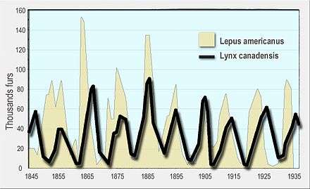
The model was later extended to include density-dependent prey growth and a functional response of the form developed by C. S. Holling; a model that has become known as the Rosenzweig–MacArthur model.[13] Both the Lotka–Volterra and Rosenzweig–MacArthur models have been used to explain the dynamics of natural populations of predators and prey, such as the lynx and snowshoe hare data of the Hudson's Bay Company[14] and the moose and wolf populations in Isle Royale National Park.[15]
In the late 1980s, an alternative to the Lotka–Volterra predator–prey model (and its common-prey-dependent generalizations) emerged, the ratio dependent or Arditi–Ginzburg model.[16] The validity of prey- or ratio-dependent models has been much debated.[17]
The Lotka–Volterra equations have a long history of use in economic theory; their initial application is commonly credited to Richard Goodwin in 1965[18] or 1967.[19][20]
Physical meaning of the equations
The Lotka–Volterra model makes a number of assumptions, not necessarily realizable in nature, about the environment and evolution of the predator and prey populations:[21]
- The prey population finds ample food at all times.
- The food supply of the predator population depends entirely on the size of the prey population.
- The rate of change of population is proportional to its size.
- During the process, the environment does not change in favour of one species, and genetic adaptation is inconsequential.
- Predators have limitless appetite.
As differential equations are used, the solution is deterministic and continuous. This, in turn, implies that the generations of both the predator and prey are continually overlapping.[22]
Prey
When multiplied out, the prey equation becomes

The prey are assumed to have an unlimited food supply and to reproduce exponentially, unless subject to predation; this exponential growth is represented in the equation above by the term αx. The rate of predation upon the prey is assumed to be proportional to the rate at which the predators and the prey meet, this is represented above by βxy. If either x or y is zero, then there can be no predation.
With these two terms the equation above can be interpreted as follows: the rate of change of the prey's population is given by its own growth rate minus the rate at which it is preyed upon.
Predators
The predator equation becomes

In this equation, δxy represents the growth of the predator population. (Note the similarity to the predation rate; however, a different constant is used, as the rate at which the predator population grows is not necessarily equal to the rate at which it consumes the prey). γy represents the loss rate of the predators due to either natural death or emigration, it leads to an exponential decay in the absence of prey.
Hence the equation expresses that the rate of change of the predator's population depends upon the rate at which it consumes prey, minus its intrinsic death rate.
Solutions to the equations
The equations have periodic solutions and do not have a simple expression in terms of the usual trigonometric functions, although they are quite tractable.[23][24]
If none of the non-negative parameters α, β, γ, δ vanishes, three can be absorbed into the normalization of variables to leave only one parameter: since the first equation is homogeneous in x, and the second one in y, the parameters β/α and δ/γ are absorbable in the normalizations of y and x respectively, and γ into the normalization of t, so that only α/γ remains arbitrary. It is the only parameter affecting the nature of the solutions.
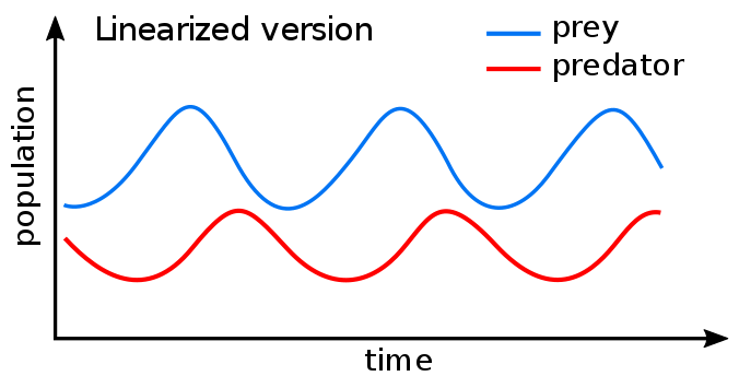
A linearization of the equations yields a solution similar to simple harmonic motion[25] with the population of predators trailing that of prey by 90° in the cycle.
A simple example
.svg.png)
Suppose there are two species of animals, a baboon (prey) and a cheetah (predator). If the initial conditions are 10 baboons and 10 cheetahs, one can plot the progression of the two species over time; given the parameters that the growth and death rates of baboon are 1.1 and 0.4 while that of cheetahs are 0.1 and 0.4 respectively. The choice of time interval is arbitrary.
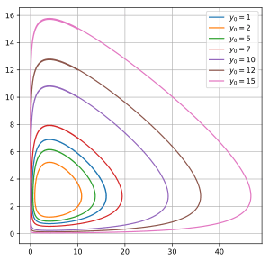
One may also plot solutions parametrically as orbits in phase space, without representing time, but with one axis representing the number of prey and the other axis representing the number of predators for all times.
This corresponds to eliminating time from the two differential equations above to produce a single differential equation

relating the variables x and y. The solutions of this equation are closed curves. It is amenable to separation of variables: integrating

yields the implicit relationship

where V is a constant quantity depending on the initial conditions and conserved on each curve.
An aside: These graphs illustrate a serious potential problem with this as a biological model: For this specific choice of parameters, in each cycle, the baboon population is reduced to extremely low numbers, yet recovers (while the cheetah population remains sizeable at the lowest baboon density). In real-life situations, however, chance fluctuations of the discrete numbers of individuals, as well as the family structure and life-cycle of baboons, might cause the baboons to actually go extinct, and, by consequence, the cheetahs as well. This modelling problem has been called the "atto-fox problem", an atto-fox being a notional 10−18 of a fox.[26][27]
Phase-space plot of a further example
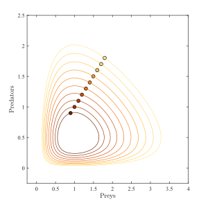
A less extreme example covers:
α = 2/3, β = 4/3, γ = 1 = δ. Assume x, y quantify thousands each. Circles represent prey and predator initial conditions from x = y = 0.9 to 1.8, in steps of 0.1. The fixed point is at (1, 1/2).
Dynamics of the system
In the model system, the predators thrive when there are plentiful prey but, ultimately, outstrip their food supply and decline. As the predator population is low, the prey population will increase again. These dynamics continue in a cycle of growth and decline.
Population equilibrium
Population equilibrium occurs in the model when neither of the population levels is changing, i.e. when both of the derivatives are equal to 0:


The above system of equations yields two solutions:

and

Hence, there are two equilibria.
The first solution effectively represents the extinction of both species. If both populations are at 0, then they will continue to be so indefinitely. The second solution represents a fixed point at which both populations sustain their current, non-zero numbers, and, in the simplified model, do so indefinitely. The levels of population at which this equilibrium is achieved depend on the chosen values of the parameters α, β, γ, and δ.
Stability of the fixed points
The stability of the fixed point at the origin can be determined by performing a linearization using partial derivatives.
The Jacobian matrix of the predator–prey model is

and is known as the community matrix.
First fixed point (extinction)
When evaluated at the steady state of (0, 0), the Jacobian matrix J becomes

The eigenvalues of this matrix are

In the model α and γ are always greater than zero, and as such the sign of the eigenvalues above will always differ. Hence the fixed point at the origin is a saddle point.
The stability of this fixed point is of significance. If it were stable, non-zero populations might be attracted towards it, and as such the dynamics of the system might lead towards the extinction of both species for many cases of initial population levels. However, as the fixed point at the origin is a saddle point, and hence unstable, it follows that the extinction of both species is difficult in the model. (In fact, this could only occur if the prey were artificially completely eradicated, causing the predators to die of starvation. If the predators were eradicated, the prey population would grow without bound in this simple model.) The populations of prey and predator can get infinitesimally close to zero and still recover.
Second fixed point (oscillations)
Evaluating J at the second fixed point leads to

The eigenvalues of this matrix are

As the eigenvalues are both purely imaginary and conjugate to each others, this fixed point is elliptic, so the solutions are periodic, oscillating on a small ellipse around the fixed point, with a frequency and period .


As illustrated in the circulating oscillations in the figure above, the level curves are closed orbits surrounding the fixed point: the levels of the predator and prey populations cycle and oscillate without damping around the fixed point with frequency .

The value of the constant of motion V, or, equivalently, K = exp(V), , can be found for the closed orbits near the fixed point.

Increasing K moves a closed orbit closer to the fixed point. The largest value of the constant K is obtained by solving the optimization problem

The maximal value of K is thus attained at the stationary (fixed) point and amounts to


where e is Euler's number.
See also
- Competitive Lotka–Volterra equations
- Generalized Lotka–Volterra equation
- Mutualism and the Lotka–Volterra equation
- Community matrix
- Population dynamics
- Population dynamics of fisheries
- Nicholson–Bailey model
- Reaction–diffusion system
- Paradox of enrichment
- Lanchester's laws, a similar system of differential equations for military forces
Notes
- Freedman, H. I. (1980). Deterministic Mathematical Models in Population Ecology. Marcel Dekker.
- Brauer, F.; Castillo-Chavez, C. (2000). Mathematical Models in Population Biology and Epidemiology. Springer-Verlag.
- Hoppensteadt, F. (2006). "Predator-prey model". Scholarpedia. 1 (10): 1563. doi:10.4249/scholarpedia.1563.
- Lotka, A. J. (1910). "Contribution to the Theory of Periodic Reaction". J. Phys. Chem. 14 (3): 271–274. doi:10.1021/j150111a004.
- Goel, N. S.; et al. (1971). On the Volterra and Other Non-Linear Models of Interacting Populations. Academic Press.
- Berryman, A. A. (1992). "The Origins and Evolution of Predator-Prey Theory" (PDF). Ecology. 73 (5): 1530–1535. doi:10.2307/1940005. JSTOR 1940005. Archived from the original (PDF) on 2010-05-31.
- Verhulst, P. H. (1838). "Notice sur la loi que la population poursuit dans son accroissement". Corresp. Mathématique et Physique. 10: 113–121.
- Lotka, A. J. (1920). "Analytical Note on Certain Rhythmic Relations in Organic Systems". Proc. Natl. Acad. Sci. U.S.A. 6 (7): 410–415. doi:10.1073/pnas.6.7.410. PMC 1084562. PMID 16576509.
- Lotka, A. J. (1925). Elements of Physical Biology. Williams and Wilkins.
- Volterra, V. (1926). "Variazioni e fluttuazioni del numero d'individui in specie animali conviventi". Mem. Acad. Lincei Roma. 2: 31–113.
- Volterra, V. (1931). "Variations and fluctuations of the number of individuals in animal species living together". In Chapman, R. N. (ed.). Animal Ecology. McGraw–Hill.
- Kingsland, S. (1995). Modeling Nature: Episodes in the History of Population Ecology. University of Chicago Press. ISBN 978-0-226-43728-6.
- Rosenzweig, M. L.; MacArthur, R.H. (1963). "Graphical representation and stability conditions of predator-prey interactions". American Naturalist. 97 (895): 209–223. doi:10.1086/282272.
- Gilpin, M. E. (1973). "Do hares eat lynx?". American Naturalist. 107 (957): 727–730. doi:10.1086/282870.
- Jost, C.; Devulder, G.; Vucetich, J.A.; Peterson, R.; Arditi, R. (2005). "The wolves of Isle Royale display scale-invariant satiation and density dependent predation on moose". J. Anim. Ecol. 74 (5): 809–816. doi:10.1111/j.1365-2656.2005.00977.x.
- Arditi, R.; Ginzburg, L. R. (1989). "Coupling in predator-prey dynamics: ratio dependence" (PDF). Journal of Theoretical Biology. 139 (3): 311–326. doi:10.1016/s0022-5193(89)80211-5.
- Abrams, P. A.; Ginzburg, L. R. (2000). "The nature of predation: prey dependent, ratio dependent or neither?". Trends in Ecology & Evolution. 15 (8): 337–341. doi:10.1016/s0169-5347(00)01908-x.
- Gandolfo, G. (2008). "Giuseppe Palomba and the Lotka–Volterra equations". Rendiconti Lincei. 19 (4): 347–357. doi:10.1007/s12210-008-0023-7.
- Goodwin, R. M. (1967). "A Growth Cycle". In Feinstein, C. H. (ed.). Socialism, Capitalism and Economic Growth. Cambridge University Press.
- Desai, M.; Ormerod, P. (1998). "Richard Goodwin: A Short Appreciation" (PDF). The Economic Journal. 108 (450): 1431–1435. CiteSeerX 10.1.1.423.1705. doi:10.1111/1468-0297.00350. Archived from the original (PDF) on 2011-09-27. Retrieved 2010-03-22.
- "PREDATOR-PREY DYNAMICS". www.tiem.utk.edu. Retrieved 2018-01-09.
- Cooke, D.; Hiorns, R. W.; et al. (1981). The Mathematical Theory of the Dynamics of Biological Populations. II. Academic Press.
- Steiner, Antonio; Gander, Martin Jakob (1999). "Parametrische Lösungen der Räuber-Beute-Gleichungen im Vergleich". Il Volterriano. 7: 32–44.
- Evans, C. M.; Findley, G. L. (1999). "A new transformation for the Lotka-Volterra problem". Journal of Mathematical Chemistry. 25: 105–110. doi:10.1023/A:1019172114300.
- Tong, H. (1983). Threshold Models in Non-linear Time Series Analysis. Springer–Verlag.
- Lobry, Claude; Sari, Tewfik (2015). "Migrations in the Rosenzweig-MacArthur model and the "atto-fox" problem" (PDF). Arima. 20: 95–125.
- Mollison, D. (1991). "Dependence of epidemic and population velocities on basic parameters" (PDF). Math. Biosci. 107 (2): 255–287. doi:10.1016/0025-5564(91)90009-8.
References
- Leigh, E. R. (1968). "The ecological role of Volterra's equations". Some Mathematical Problems in Biology. – a modern discussion using Hudson's Bay Company data on lynx and hares in Canada from 1847 to 1903.
- Kaplan, Daniel; Glass, Leon (1995). Understanding Nonlinear Dynamics. New York: Springer. ISBN 978-0-387-94440-1.
- Murray, J. D. (2003). Mathematical Biology I: An Introduction. New York: Springer. ISBN 978-0-387-95223-9.
- Yorke, James A.; Anderson, William N. Jr. (1973). "Predator-Prey Patterns (Volterra-Lotka equations)" (PDF). PNAS. 70 (7): 2069–2071. doi:10.1073/pnas.70.7.2069. JSTOR 62597. PMID 16592100.
- Llibre, J.; Valls, C. (2007). "Global analytic first integrals for the real planar Lotka-Volterra system". J. Math. Phys. 48 (3): 033507. doi:10.1063/1.2713076.
External links
| Wikimedia Commons has media related to Lotka-Volterra equations. |
- From the Wolfram Demonstrations Project — requires CDF player (free):
- Lotka-Volterra Algorithmic Simulation (Web simulation).