Vorticity

In a mass of continuum that is rotating like a rigid body, the vorticity is twice the angular velocity vector of that rotation. This is the case, for example, in the central core of a Rankine vortex.

The vorticity may be nonzero even when all particles are flowing along straight and parallel pathlines, if there is shear (that is, if the flow speed varies across streamlines). For example, in the laminar flow within a pipe with constant cross section, all particles travel parallel to the axis of the pipe; but faster near that axis, and practically stationary next to the walls. The vorticity will be zero on the axis, and maximum near the walls, where the shear is largest.

Conversely, a flow may have zero vorticity even though its particles travel along curved trajectories. An example is the ideal irrotational vortex, where most particles rotate about some straight axis, with speed inversely proportional to their distances to that axis. A small parcel of continuum that does not straddle the axis will be rotated in one sense but sheared in the opposite sense, in such a way that their mean angular velocity about their center of mass is zero.

Example flows:
Rigid-body-like vortex v ∝ r	Parallel flow with shear	Irrotational vortex v ∝ 1/r
where v is the velocity of the flow, r is the distance to the center of the vortex and ∝ indicates proportionality. Absolute velocities around the highlighted point: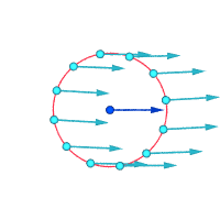
Relative velocities (magnified) around the highlighted point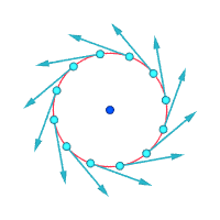
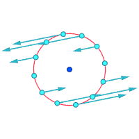
Vorticity ≠ 0	Vorticity ≠ 0	Vorticity = 0

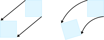
Another way to visualize vorticity is to imagine that, instantaneously, a tiny part of the continuum becomes solid and the rest of the flow disappears. If that tiny new solid particle is rotating, rather than just moving with the flow, then there is vorticity in the flow. In the figure below, the left subfigure demonstrates no vorticity, and the right subfigure demonstrates existence of vorticity.

Mathematically, the vorticity of a three-dimensional flow is a pseudovector field, usually denoted by ω→, defined as the curl or rotational of the velocity field v→ describing the continuum motion. In Cartesian coordinates:

${\displaystyle {\begin{aligned}{\vec {\omega }}=\nabla \times {\vec {v}}&={\begin{pmatrix}{\frac {\partial }{\partial x}}&{\frac {\partial }{\partial y}}&{\frac {\partial }{\partial z}}\end{pmatrix}}\times {\begin{pmatrix}v_{x}&v_{y}&v_{z}\end{pmatrix}}\\[6px]&={\begin{pmatrix}{\frac {\partial v_{z}}{\partial y}}-{\frac {\partial v_{y}}{\partial z}}&{\frac {\partial v_{x}}{\partial z}}-{\frac {\partial v_{z}}{\partial x}}&{\frac {\partial v_{y}}{\partial x}}-{\frac {\partial v_{x}}{\partial y}}\end{pmatrix}}\,.\end{aligned}}}$

In words, the vorticity tells how the velocity vector changes when one moves by an infinitesimal distance in a direction perpendicular to it.

In a two-dimensional flow where the velocity is independent of the z coordinate and has no z component, the vorticity vector is always parallel to the z axis, and therefore can be expressed as a scalar field multiplied by a constant unit vector z→:

${\displaystyle {\begin{aligned}{\vec {\omega }}=\nabla \times {\vec {v}}&={\begin{pmatrix}{\frac {\partial }{\partial x}}&{\frac {\partial }{\partial y}}&{\frac {\partial }{\partial z}}\end{pmatrix}}\times \left(v_{x},v_{y},0\right)\\[6px]&=\left({\frac {\partial v_{y}}{\partial x}}-{\frac {\partial v_{x}}{\partial y}}\right){\vec {z}}\,.\end{aligned}}}$

The evolution of the vorticity field in time is described by the vorticity equation, which can be derived from the Navier–Stokes equations.

In many real flows where the viscosity can be neglected (more precisely, in flows with high Reynolds number), the vorticity field can be modeled well by a collection of discrete vortices, the vorticity being negligible everywhere except in small regions of space surrounding the axes of the vortices. This is clearly true in the case of two-dimensional potential flow (i.e. two-dimensional zero viscosity flow), in which case the flowfield can be modeled as a complex-valued field on the complex plane.

Vorticity is a useful tool to understand how the ideal potential flow solutions can be perturbed to model real flows. In general, the presence of viscosity causes a diffusion of vorticity away from the vortex cores into the general flow field. This flow is accounted for by the diffusion term in the vorticity transport equation. Thus, in cases of very viscous flows (e.g. Couette Flow), the vorticity will be diffused throughout the flow field and it is probably simpler to look at the velocity field than at the vorticity.

A vortex line or vorticity line is a line which is everywhere tangent to the local vorticity vector. Vortex lines are defined by the relation[3]

${\displaystyle {\frac {dx}{\omega _{x}}}={\frac {dy}{\omega _{y}}}={\frac {dz}{\omega _{z}}}\,,}$

where ω→ = (ω_x, ω_y, ω_z) is the vorticity vector in Cartesian coordinates.

A vortex tube is the surface in the continuum formed by all vortex lines passing through a given (reducible) closed curve in the continuum. The 'strength' of a vortex tube (also called vortex flux)[4] is the integral of the vorticity across a cross-section of the tube, and is the same everywhere along the tube (because vorticity has zero divergence). It is a consequence of Helmholtz's theorems (or equivalently, of Kelvin's circulation theorem) that in an inviscid fluid the 'strength' of the vortex tube is also constant with time. Viscous effects introduce frictional losses and time dependence.

In a three-dimensional flow, vorticity (as measured by the volume integral of the square of its magnitude) can be intensified when a vortex line is extended — a phenomenon known as vortex stretching.[5] This phenomenon occurs in the formation of a bathtub vortex in outflowing water, and the build-up of a tornado by rising air currents.

Helicity is vorticity in motion along a third axis in a corkscrew fashion.

• Barotropic vorticity equation
• D'Alembert's paradox
• Enstrophy
• Velocity potential
• Vortex
• Vortex tube
• Vortex stretching
• Vortical
• Horseshoe vortex
• Wingtip vortices

• Clancy, L.J. (1975), Aerodynamics, Pitman Publishing Limited, London ISBN 0-273-01120-0
• "Weather Glossary"' The Weather Channel Interactive, Inc.. 2004.
• "Vorticity". Integrated Publishing.

• Batchelor, G. K. (2000) [1967], An Introduction to Fluid Dynamics, Cambridge University Press, ISBN 0-521-66396-2
• Ohkitani, K., "Elementary Account Of Vorticity And Related Equations". Cambridge University Press. January 30, 2005. ISBN 0-521-81984-9
• Chorin, Alexandre J., "Vorticity and Turbulence". Applied Mathematical Sciences, Vol 103, Springer-Verlag. March 1, 1994. ISBN 0-387-94197-5
• Majda, Andrew J., Andrea L. Bertozzi, "Vorticity and Incompressible Flow". Cambridge University Press; 2002. ISBN 0-521-63948-4
• Tritton, D. J., "Physical Fluid Dynamics". Van Nostrand Reinhold, New York. 1977. ISBN 0-19-854493-6
• Arfken, G., "Mathematical Methods for Physicists", 3rd ed. Academic Press, Orlando, Florida. 1985. ISBN 0-12-059820-5

Wikimedia Commons has media related to Vorticity.

• Weisstein, Eric W., "Vorticity". Scienceworld.wolfram.com.
• Doswell III, Charles A., "A Primer on Vorticity for Application in Supercells and Tornadoes". Cooperative Institute for Mesoscale Meteorological Studies, Norman, Oklahoma.
• Cramer, M. S., "Navier–Stokes Equations -- Vorticity Transport Theorems: Introduction". Foundations of Fluid Mechanics.
• Parker, Douglas, "ENVI 2210 - Atmosphere and Ocean Dynamics, 9: Vorticity". School of the Environment, University of Leeds. September 2001.
• Graham, James R., "Astronomy 202: Astrophysical Gas Dynamics". Astronomy Department, UC Berkeley.
  • "The vorticity equation: incompressible and barotropic fluids".
  • "Interpretation of the vorticity equation".
  • "Kelvin's vorticity theorem for incompressible or barotropic flow".
• "Spherepack 3.1". (includes a collection of FORTRAN vorticity program)
• "Mesoscale Compressible Community (MC2) Real-Time Model Predictions". (Potential vorticity analysis)

References

- Lecture Notes from University of Washington Archived October 16, 2015, at the Wayback Machine
- Clancy, L.J., Aerodynamics, Section 7.11
- Kundu P and Cohen I. Fluid Mechanics.
- Introduction to Astrophysical Gas Dynamics Archived June 14, 2011, at the Wayback Machine
- Batchelor, section 5.2
- Joukovsky N.E. (1914). "On the motion of water at a turn of a river". Matematicheskii Sbornik. 28.. Reprinted in: Collected works. 4. Moscow; Leningrad. 1937. pp. 193–216, 231–233 (abstract in English). "Professor Milovich's float", as Joukovsky refers this vorticity meter to, is schematically shown in figure on page 196 of Collected works.
- National Committee for Fluid Mechanics Films Archived October 21, 2016, at the Wayback Machine
- Films by Hunter Rouse — IIHR — Hydroscience & Engineering Archived April 21, 2016, at the Wayback Machine