Hagen–Poiseuille equation
In nonideal fluid dynamics, the Hagen–Poiseuille equation, also known as the Hagen–Poiseuille law, Poiseuille law or Poiseuille equation, is a physical law that gives the pressure drop in an incompressible and Newtonian fluid in laminar flow flowing through a long cylindrical pipe of constant cross section. It can be successfully applied to air flow in lung alveoli, or the flow through a drinking straw or through a hypodermic needle. It was experimentally derived independently by Jean Léonard Marie Poiseuille in 1838[1] and Gotthilf Heinrich Ludwig Hagen,[2] and published by Poiseuille in 1840–41 and 1846.[1] The theoretical justification of the Poiseuille law was given by George Stokes in 1845.[3]
| Part of a series on | |||||||
| Continuum mechanics | |||||||
|---|---|---|---|---|---|---|---|
|
Laws
|
|||||||
|
|||||||
The assumptions of the equation are that the fluid is incompressible and Newtonian; the flow is laminar through a pipe of constant circular cross-section that is substantially longer than its diameter; and there is no acceleration of fluid in the pipe. For velocities and pipe diameters above a threshold, actual fluid flow is not laminar but turbulent, leading to larger pressure drops than calculated by the Hagen–Poiseuille equation.
Poiseuille's Equation describes the pressure drop due to the viscosity of the fluid; Other types of pressure drops may still occur in a fluid (see a demonstration here[4]). For example, the pressure needed to drive a viscous fluid up against gravity would contain both that as needed in Poiseuille's Law plus that as needed in Bernoulli's equation, such that any point in the flow would have a pressure greater than zero (otherwise no flow would happen).
Another example is when blood flows into a narrower constriction, its speed will be greater than in a larger diameter (due to continuity of volumetric flow rate), and its pressure will be lower than in a larger diameter[4] (due to Bernoulli's equation). However, the viscosity of blood will also cause additional pressure drop along the direction of flow, which is proportional to length traveled[4] (as per Poiseuille's Law). Both effects contribute to the actual pressure drop.
Equation
In standard fluid-kinetics notation:[5][6][7]

where:
- Δp is the pressure difference between the two ends,
- L is the length of pipe,
- μ is the dynamic viscosity,
- Q is the volumetric flow rate,
- R is the pipe radius,
- A is the cross section of pipe.
The equation does not hold close to the pipe entrance.[8]:3
The equation fails in the limit of low viscosity, wide and/or short pipe. Low viscosity or a wide pipe may result in turbulent flow, making it necessary to use more complex models, such as Darcy–Weisbach equation. The ratio of length to radius of a pipe should be greater than one forty-eighth of the Reynolds number for the Hagen-Poiseuille law to be valid.[9] If the pipe is too short, the Hagen–Poiseuille equation may result in unphysically high flow rates; the flow is bounded by Bernoulli's principle, under less restrictive conditions, by

because it's impossible to have less-than-zero (absolute) pressure (not to be confused with gauge pressure) in an incompressible flow.
Relation to Darcy–Weisbach
Normally, Hagen–Poiseuille flow implies not just the relation for the pressure drop, above, but also the full solution for the laminar flow profile, which is parabolic. However, the result for the pressure drop can be extended to turbulent flow by inferring an effective turbulent viscosity in the case of turbulent flow, even though the flow profile in turbulent flow is strictly speaking not actually parabolic. In both cases, laminar or turbulent, the pressure drop is related to the stress at the wall, which determines the so-called friction factor. The wall stress can be determined phenomenologically by the Darcy–Weisbach equation in the field of hydraulics, given a relationship for the friction factor in terms of the Reynolds number. In the case of laminar flow, for a circular cross section:

where Re is the Reynolds number, ρ is the fluid density, and v is the mean flow velocity, which is half the maximal flow velocity in the case of laminar flow. It proves more useful to define the Reynolds number in terms of the mean flow velocity because this quantity remains well defined even in the case of turbulent flow, whereas the maximal flow velocity may not be, or in any case, it may be difficult to infer. In this form the law approximates the Darcy friction factor, the energy (head) loss factor, friction loss factor or Darcy (friction) factor Λ in the laminar flow at very low velocities in cylindrical tube. The theoretical derivation of a slightly different form of the law was made independently by Wiedman in 1856 and Neumann and E. Hagenbach in 1858 (1859, 1860). Hagenbach was the first who called this law the Poiseuille's law.
The law is also very important in hemorheology and hemodynamics, both fields of physiology.[10]
Poiseuille's law was later in 1891 extended to turbulent flow by L. R. Wilberforce, based on Hagenbach's work.
Derivation
The Hagen–Poiseuille equation can be derived from the Navier–Stokes equations. The laminar flow through a pipe of uniform (circular) cross-section is known as Hagen–Poiseuille flow. The equations governing the Hagen–Poiseuille flow can be derived directly from the Navier–Stokes momentum equations in 3D cylindrical coordinates by making the following set of assumptions:

- The flow is steady ( ).
- The radial and azimuthal components of the fluid velocity are zero ( ).
- The flow is axisymmetric ( ).
- The flow is fully developed ( ). Here However, this can be proved via mass conservation, and the above assumptions.


Then the angular equation in the momentum equations and the continuity equation are identically satisfied. The radial momentum equation reduces to , i.e., the pressure is a function of the axial coordinate only. For brevity, use instead of . The axial momentum equation reduces to


where is the dynamic viscosity of the fluid. In the above equation, the left-hand side is only a function of and the right-hand side term is only a function of , implying that both terms must be the same constant. Evaluating this constant is straightforward. If we take the length of the pipe to be and denote the pressure difference between the two ends of the pipe by (high pressure minus low pressure), then the constant is simply defined such that is positive. The solution is


Since needs to be finite at , . The no slip boundary condition at the pipe wall requires that at (radius of the pipe), which yields Thus we have finally the following parabolic velocity profile:


The maximum velocity occurs at the pipe centerline (), . The average velocity can be obtained by integrating over the pipe cross section,


The easily measurable quantity in experiments is the volumetric flow rate . Rearrangement of this gives the Hagen–Poiseuille equation


Elaborate derivation starting directly from first principles Although more lengthy than directly using the Navier–Stokes equations, an alternative method of deriving the Hagen–Poiseuille equation is as follows. Liquid flow through a pipe
Assume the liquid exhibits laminar flow. Laminar flow in a round pipe prescribes that there are a bunch of circular layers (lamina) of liquid, each having a velocity determined only by their radial distance from the center of the tube. Also assume the center is moving fastest while the liquid touching the walls of the tube is stationary (due to the no-slip condition).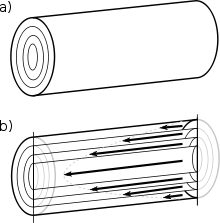 a) A tube showing the imaginary lamina. b) A cross section of the tube shows the lamina moving at different speeds. Those closest to the edge of the tube are moving slowly while those near the center are moving quickly.
To figure out the motion of the liquid, all forces acting on each lamina must be known:
- The pressure force pushing the liquid through the tube is the change in pressure multiplied by the area: F = −A Δp. This force is in the direction of the motion of the liquid. The negative sign comes from the conventional way we define Δp = pend − ptop < 0.
- Viscosity effects will pull from the faster lamina immediately closer to the center of the tube.
- Viscosity effects will drag from the slower lamina immediately closer to the walls of the tube.
Viscosity
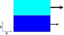 Two fluids moving past each other in the x direction. The liquid on top is moving faster and will be pulled in the negative direction by the bottom liquid while the bottom liquid will be pulled in the positive direction by the top liquid.
When two layers of liquid in contact with each other move at different speeds, there will be a shear force between them. This force is proportional to the area of contact A, the velocity gradient perpendicular to the direction of flow Δvx/Δy, and a proportionality constant (viscosity) and is given by
The negative sign is in there because we are concerned with the faster moving liquid (top in figure), which is being slowed by the slower liquid (bottom in figure). By Newton's third law of motion, the force on the slower liquid is equal and opposite (no negative sign) to the force on the faster liquid. This equation assumes that the area of contact is so large that we can ignore any effects from the edges and that the fluids behave as Newtonian fluids.
Faster lamina
Assume that we are figuring out the force on the lamina with radius r. From the equation above, we need to know the area of contact and the velocity gradient. Think of the lamina as a ring of radius r, thickness dr, and length Δx. The area of contact between the lamina and the faster one is simply the area of the inside of the cylinder: A = 2πr Δx. We don't know the exact form for the velocity of the liquid within the tube yet, but we do know (from our assumption above) that it is dependent on the radius. Therefore, the velocity gradient is the change of the velocity with respect to the change in the radius at the intersection of these two laminae. That intersection is at a radius of r. So, considering that this force will be positive with respect to the movement of the liquid (but the derivative of the velocity is negative), the final form of the equation becomes
where the vertical bar and subscript r following the derivative indicates that it should be taken at a radius of r.
Slower lamina
Next let's find the force of drag from the slower lamina. We need to calculate the same values that we did for the force from the faster lamina. In this case, the area of contact is at r + dr instead of r. Also, we need to remember that this force opposes the direction of movement of the liquid and will therefore be negative (and that the derivative of the velocity is negative).
Putting it all together
To find the solution for the flow of a laminar layer through a tube, we need to make one last assumption. There is no acceleration of liquid in the pipe, and by Newton's first law, there is no net force. If there is no net force then we can add all of the forces together to get zero
or
First, to get everything happening at the same point, use the first two terms of a Taylor series expansion of the velocity gradient:
The expression is valid for all laminae. Grouping like terms and dropping the vertical bar since all derivatives are assumed to be at radius r,
Finally, put this expression in the form of a differential equation, dropping the term quadratic in dr.
The above equation is the same as the one obtained from the Navier-Stokes equations and the derivation from here on follows as before.


Startup of Poiseuille flow in a pipe[11]
When a constant pressure gradient is applied between two ends of a long pipe, the flow will not immediately obtain Poiseuille profile, rather it develops through time and reaches the Poiseuille profile at steady state. The Navier-Stokes equations reduce to


with initial and boundary conditions,

The velocity distribution is given by

where is the Bessel function of the first kind of order zero and are the positive roots of this function and is the Bessel function of the first kind of order one. As , Poiseuille solution is recovered.


Poiseuille flow in annular section[12]
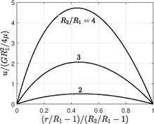
If is the inner cylinder radii and is the outer cylinder radii, with applied pressure gradient between the two ends , the velocity distribution and the volume flux through the annular pipe are


When , the original problem is recovered.

Poiseuille flow in a pipe with oscillating pressure gradient
Flow through pipes with oscillating pressure gradient finds applications in blood flow through large arteries[13][14][15][16]. The imposed pressure gradient is given by

where , and are constants and is the frequency. The velocity field is given by


where


where and are the Kelvin functions and .


Plane Poiseuille flow
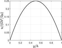
Plane Poiseuille flow is flow created between two infinitely long parallel plates, separated by a distance with a constant pressure gradient is applied in the direction of flow. The flow is essentially unidirectional because of infinite length. The Navier-Stokes equations reduce to


with no-slip condition on both walls

Therefore, the velocity distribution and the volume flow rate per unit length are

Poiseuille flow through some non-circular cross-sections[17]
Joseph Boussinesq[18] derived the velocity profile and volume flow rate in 1868 for rectangular channel and tubes of equilateral triangular cross-section and for elliptical cross-section. Joseph Proudman[19] derived the same for isosceles triangles in 1914. Let be the constant pressure gradient acting in direction parallel to the motion.
The velocity and the volume flow rate in a rectangular channel of height and width are


The velocity and the volume flow rate of tube with equilateral triangular cross-section of side length are


The velocity and the volume flow rate in the right-angled isosceles triangle are


The velocity distribution for tubes of elliptical cross-section with semi-axis and is[11]


Here, when , Poiseuille flow for circular pipe is recovered and when , plane Poiseuille flow is recovered. More explicit solutions with cross-sections such as snail-shaped sections, sections having the shape of a notch circle following a semicircle, annular sections between homofocal ellipses, annular sections between non-concentric circles are also available, as reviewed by Ratip Berker.[20]


Poiseuille flow through arbitrary cross-section
The flow through arbitrary cross-section satisfies the condition that on the walls. The governing equation reduces to[21]


If we introduce a new dependent variable as

then it is easy to see that the problem reduces to that integrating a Laplace equation

satisfying the condition

on the wall.
Poiseuille's equation for an ideal isothermal gas
For a compressible fluid in a tube the volumetric flow rate (but not the mass flow rate) and the axial velocity are not constant along the tube. The flow is usually expressed at outlet pressure. As fluid is compressed or expands, work is done and the fluid is heated or cooled. This means that the flow rate depends on the heat transfer to and from the fluid. For an ideal gas in the isothermal case, where the temperature of the fluid is permitted to equilibrate with its surroundings, an approximate relation for the pressure drop can be derived.[22] Using ideal gas equation of state for constant temperature process, the relation can be obtained. Over a short section of the pipe, the gas flowing through the pipe can be assumed to be incompressible so that Poiseuille law can be used locally,


Here we assumed the local pressure gradient is not too great to have any compressibility effects. Though locally we ignored the effects of pressure variation due to density variation, over long distances these effects are taken into account. Since is independent of pressure, the above equation can be integrated over the length to give

Hence the volumetric flow rate at the pipe outlet is given by

This equation can be seen as Poiseuille's law with an extra correction factor p1 + p2/2p2 expressing the average pressure relative to the outlet pressure.
Electrical circuits analogy
Electricity was originally understood to be a kind of fluid. This hydraulic analogy is still conceptually useful for understanding circuits. This analogy is also used to study the frequency response of fluid-mechanical networks using circuit tools, in which case the fluid network is termed a hydraulic circuit. Poiseuille's law corresponds to Ohm's law for electrical circuits, V = IR. Since the net force acting on the fluid is equal to , where S = πr2, i.e. ΔF = πr2 ΔP, then from Poiseuille's law, it follows that

- .

For electrical circuits, let n be the concentration of free charged particles (in m−3) and let q* be the charge of each particle (in coulombs). (For electrons, q* = e = 1.6×10⁻¹⁹ C.) Then nQ is the number of particles in the volume Q, and nQq* is their total charge. This is the charge that flows through the cross section per unit time, i.e. the current I. Therefore, I = nQq*. Consequently, Q = I/nq*, and

But ΔF = Eq, where q is the total charge in the volume of the tube. The volume of the tube is equal to πr2L, so the number of charged particles in this volume is equal to nπr2L, and their total charge is Since the voltage V = EL, it follows then


This is exactly Ohm's law, where the resistance R = V/I is described by the formula
- .

It follows that the resistance R is proportional to the length L of the resistor, which is true. However, it also follows that the resistance R is inversely proportional to the fourth power of the radius r, i.e. the resistance R is inversely proportional to the second power of the cross section area S = πr2 of the resistor, which is wrong according to the electrical analogy. The correct relation is

where ρ is the specific resistance; i.e. the resistance R is inversely proportional to the cross section area S of the resistor.[23] The reason why Poiseuille's law leads to a wrong formula for the resistance R is the difference between the fluid flow and the electric current. Electron gas is inviscid, so its velocity does not depend on the distance to the walls of the conductor. The resistance is due to the interaction between the flowing electrons and the atoms of the conductor. Therefore, Poiseuille's law and the hydraulic analogy are useful only within certain limits when applied to electricity. Both Ohm's law and Poiseuille's law illustrate transport phenomena.
Medical applications – intravenous access and fluid delivery
The Hagen–Poiseuille equation is useful in determining the vascular resistance and hence flow rate of intravenous fluids that may be achieved using various sizes of peripheral and central cannulas. The equation states that flow rate is proportional to the radius to the fourth power, meaning that a small increase in the internal diameter of the cannula yields a significant increase in flow rate of IV fluids. The radius of IV cannulas is typically measured in "gauge", which is inversely proportional to the radius. Peripheral IV cannulas are typically available as (from large to small) 14G, 16G, 18G, 20G, 22G. As an example, the flow of a 14G cannula is typically twice that of a 16G, and ten times that of a 20G. It also states that flow is inversely proportional to length, meaning that longer lines have lower flow rates. This is important to remember as in an emergency, many clinicians favor shorter, larger catheters compared to longer, narrower catheters. While of less clinical importance, the change in pressure can be used to speed up flow rate by pressurizing the bag of fluid, squeezing the bag, or hanging the bag higher from the level of the cannula. It is also useful to understand that viscous fluids will flow slower (e.g. in blood transfusion).
See also
- Couette flow
- Darcy's law
- Pulse
- Wave
- Hydraulic circuit
Notes
- Sutera, Salvatore P.; Skalak, Richard (1993). "The History of Poiseuille's Law". Annual Review of Fluid Mechanics. 25: 1–19. Bibcode:1993AnRFM..25....1S. doi:10.1146/annurev.fl.25.010193.000245.
- István Szabó, ;;Geschichte der mechanischen Prinzipien und ihrer wichtigsten Anwendungen, Basel: Birkhäuser Verlag, 1979.
- Stokes, G. G. (1845). On the theories of the internal friction of fluids in motion, and of the equilibrium and motion of elastic solids. Transactions of the Cambridge Philosophical Society, 8, 287-341
- "Pressure". hyperphysics.phy-astr.gsu.edu. Retrieved 2019-12-15.
- Kirby, B. J. (2010). Micro- and Nanoscale Fluid Mechanics: Transport in Microfluidic Devices. Cambridge University Press. ISBN 978-0-521-11903-0.
- Bruus, H. (2007). Theoretical Microfluidics.
- "Poiseuille and his law" (PDF). pdfs.semanticscholar.org.
- Vogel, Steven (1981). Life in Moving Fluids: The Physical Biology of Flow. PWS Kent Publishers. ISBN 0871507498.
- tec-science (2020-04-02). "Energetic analysis of the Hagen-Poiseuille law". tec-science. Retrieved 2020-05-07.
- Determinants of blood vessel resistance.
- Batchelor, George Keith. An introduction to fluid dynamics. Cambridge university press, 2000.
- Rosenhead, Louis, ed. Laminar boundary layers. Clarendon Press, 1963.
- Sexl, T. (1930). Über den von EG Richardson entdeckten „Annulareffekt “. Zeitschrift für Physik, 61(5-6), 349-362.
- Lambossy, P. (1952). Oscillations forcees d'un liquide incompressibile et visqueux dans un tube rigide et horizontal. Calcul de la force frottement. Helv. physica acta, 25, 371-386.
- Womersley, J. R. (1955). Method for the calculation of velocity, rate of flow and viscous drag in arteries when the pressure gradient is known. The Journal of physiology, 127(3), 553-563.
- Uchida, S. (1956). The pulsating viscous flow superposed on the steady laminar motion of incompressible fluid in a circular pipe. Zeitschrift für angewandte Mathematik und Physik ZAMP, 7(5), 403-422.
- Drazin, Philip G., and Norman Riley. The Navier–Stokes equations: a classification of flows and exact solutions. No. 334. Cambridge University Press, 2006.
- Boussinesq, Joseph. "Mémoire sur l’influence des Frottements dans les Mouvements Réguliers des Fluids." J. Math. Pures Appl 13.2 (1868): 377-424.
- Proudman, J. "IV. Notes on the motion of viscous liquids in channels." The London, Edinburgh, and Dublin Philosophical Magazine and Journal of Science 28.163 (1914): 30-36.
- Berker, R. (1963). Intégration des équations du mouvement d'un fluide visqueux incompressible. Handbuch der physik, 3, 1-384.
- Samuel Newby Curle and H.J. Davies. Modern Fluid Dynamics. Volume 1, Incompressible Flow, Van Nostrand Reinhold Inc (1971)
- Landau, L. D., & Lifshitz, E. M. (1987). Fluid Mechanics, Pargamon, Page 55, problem 6
- Fütterer, C. et al. "Injection and flow control system for microchannels" Lab-on-a-Chip (2004): 351-356.
References
- Sutera, S. P.; Skalak, R. (1993). "The history of Poiseuille's law". Annual Review of Fluid Mechanics. 25: 1–19. Bibcode:1993AnRFM..25....1S. doi:10.1146/annurev.fl.25.010193.000245..
- Pfitzner, J (1976). "Poiseuille and his law". Anaesthesia. 31 (2) (published Mar 1976). pp. 273–5. doi:10.1111/j.1365-2044.1976.tb11804.x. PMID 779509..
- Bennett, C. O.; Myers, J. E. (1962). "Momentum, Heat, and Mass Transfer". McGraw-Hill. Cite journal requires
|journal=(help).