Vapour pressure of water

The vapour pressure of water is the pressure at which water vapour is in thermodynamic equilibrium with its condensed state. At higher pressures water would condense. The water vapour pressure is the partial pressure of water vapour in any gas mixture in equilibrium with solid or liquid water. As for other substances, water vapour pressure is a function of temperature and can be determined with the Clausius–Clapeyron relation.

Vapour pressure of water (0–100 °C)[1]
T, °C	T, °F	P, kPa	P, torr	P, atm
0	32	0.6113	4.5851	0.0060
5	41	0.8726	6.5450	0.0086
10	50	1.2281	9.2115	0.0121
15	59	1.7056	12.7931	0.0168
20	68	2.3388	17.5424	0.0231
25	77	3.1690	23.7695	0.0313
30	86	4.2455	31.8439	0.0419
35	95	5.6267	42.2037	0.0555
40	104	7.3814	55.3651	0.0728
45	113	9.5898	71.9294	0.0946
50	122	12.3440	92.5876	0.1218
55	131	15.7520	118.1497	0.1555
60	140	19.9320	149.5023	0.1967
65	149	25.0220	187.6804	0.2469
70	158	31.1760	233.8392	0.3077
75	167	38.5630	289.2463	0.3806
80	176	47.3730	355.3267	0.4675
85	185	57.8150	433.6482	0.5706
90	194	70.1170	525.9208	0.6920
95	203	84.5290	634.0196	0.8342
100	212	101.3200	759.9625	1.0000

Approximation formulas

There are many published approximations for calculating saturated vapour pressure over water and over ice. Some of these are (in approximate order of increasing accuracy):

$P=\exp \left(20.386-{\frac {5132}{T}}\right),\ \ \ \ (Eq.1)$

where

P

is the vapour pressure in mmHg and

T

is the temperature in kelvins.

The Antoine equation

\log _{10}P=A-{\frac {B}{C+T}},

where the temperature

T

is in degrees Celsius (°C) and the vapour pressure

P

is in mmHg. The constants are given as

$A$	$B$	$C$	$T min$ , °C	$T max$ , °C
8.07131	1730.63	233.426	1	99
8.14019	1810.94	244.485	100	374

The August-Roche-Magnus (or Magnus-Tetens or Magnus) equation, as described in Alduchov and Eskridge (1996).[2] Equation 25 in [2] provides the coefficients used here. See also discussion of Clausius-Clapeyron approximations used in meteorology and climatology.

P=0.61094\exp \left({\frac {17.625T}{T+243.04}}\right),

where temperature $T$ is in °C and vapour pressure $P$ is in kilopascals (kPa)

The Tetens equation

P=0.61078\exp \left({\frac {17.27T}{T+237.3}}\right),

where temperature $T$ is in °C and $P$ is in kPa

The Buck equation.

P=0.61121\exp \left(\left(18.678-{\frac {T}{234.5}}\right)\left({\frac {T}{257.14+T}}\right)\right),

where $T$ is in °C and $P$ is in kPa.

The Goff-Gratch (1946) equation.[3]

Accuracy of different formulations

Here is a comparison of the accuracies of these different explicit formulations, showing saturation vapour pressures for liquid water in kPa, calculated at six temperatures with their percentage error from the table values of Lide (2005):

$T$ (°C)	$P$ (Lide Table)	$P$ (Eq 1)	$P$ (Antoine)	$P$ (Magnus)	$P$ (Tetens)	$P$ (Buck)	$P$ (Goff-Gratch)
0	0.6113	0.6593 (+7.85%)	0.6056 (-0.93%)	0.6109 (-0.06%)	0.6108 (-0.09%)	0.6112 (-0.01%)	0.6089 (-0.40%)
20	2.3388	2.3755 (+1.57%)	2.3296 (-0.39%)	2.3334 (-0.23%)	2.3382 (+0.05%)	2.3383 (-0.02%)	2.3355 (-0.14%)
35	5.6267	5.5696 (-1.01%)	5.6090 (-0.31%)	5.6176 (-0.16%)	5.6225 (+0.04%)	5.6268 (+0.00%)	5.6221 (-0.08%)
50	12.344	12.065 (-2.26%)	12.306 (-0.31%)	12.361 (+0.13%)	12.336 (+0.08%)	12.349 (+0.04%)	12.338 (-0.05%)
75	38.563	37.738 (-2.14%)	38.463 (-0.26%)	39.000 (+1.13%)	38.646 (+0.40%)	38.595 (+0.08%)	38.555 (-0.02%)
100	101.32	101.31 (-0.01%)	101.34 (+0.02%)	104.077 (+2.72%)	102.21 (+1.10%)	101.31 (-0.01%)	101.32 (0.00%)

A more detailed discussion of accuracy and considerations of the inaccuracy in temperature measurements is presented in Alduchov and Eskridge (1996). The analysis here shows the simple unattributed formula and the Antoine equation are reasonably accurate at 100 °C, but quite poor for lower temperatures above freezing. Tetens is much more accurate over the range from 0 to 50 °C and very competitive at 75 °C, but Antoine's is superior at 75 °C and above. The unattributed formula must have zero error at around 26 °C, but is of very poor accuracy outside a very narrow range. Tetens' equations are generally much more accurate and arguably simpler for use at everyday temperatures (e.g., in meteorology). As expected, Buck's equation for $T$ > 0 °C is significantly more accurate than Tetens, and its superiority increases markedly above 50 °C, though it is more complicated to use. The Buck equation is even superior to the more complex Goff-Gratch equation over the range needed for practical meteorology.

Numerical approximations

For serious computation, Lowe (1977)[4] developed two pairs of equations for temperatures above and below freezing, with different levels of accuracy. They are all very accurate (compared to Clausius-Clapeyron and the Goff-Gratch) but use nested polynomials for very efficient computation. However, there are more recent reviews of possibly superior formulations, notably Wexler (1976, 1977),[5][6] reported by Flatau et al. (1992).[7]

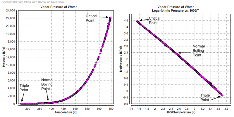
Graphical pressure dependency on temperature

Vapour pressure diagrams of water; data taken from Dortmund Data Bank. Graphics shows triple point, critical point and boiling point of water.

References

Lide, David R., ed. (2004). CRC Handbook of Chemistry and Physics, (85th ed.). CRC Press. pp. 6–8. ISBN 978-0-8493-0485-9.
Alduchov, O.A.; Eskridge, R.E. (1996). "Improved Magnus form approximation of saturation vapor pressure". Journal of Applied Meteorology. 35 (4): 601–9. Bibcode:1996JApMe..35..601A. doi:10.1175/1520-0450(1996)035<0601:IMFAOS>2.0.CO;2.
Goff, J.A., and Gratch, S. 1946. Low-pressure properties of water from −160 to 212 °F. In Transactions of the American Society of Heating and Ventilating Engineers, pp 95–122, presented at the 52nd annual meeting of the American Society of Heating and Ventilating Engineers, New York, 1946.
Lowe, P.R. (1977). "An approximating polynomial for the computation of saturation vapor pressure". Journal of Applied Meteorology. 16 (1): 100–4. Bibcode:1977JApMe..16..100L. doi:10.1175/1520-0450(1977)016<0100:AAPFTC>2.0.CO;2.
Wexler, A. (1976). "Vapor pressure formulation for water in range 0 to 100°C. A revision". Journal of Research of the National Bureau of Standards Section A. 80A (5–6): 775–785. doi:10.6028/jres.080a.071.
Wexler, A. (1977). "Vapor pressure formulation for ice". Journal of Research of the National Bureau of Standards Section A. 81A (1): 5–20. doi:10.6028/jres.081a.003.
Flatau, P.J.; Walko, R.L.; Cotton, W.R. (1992). "Polynomial fits to saturation vapor pressure". Journal of Applied Meteorology. 31 (12): 1507–13. Bibcode:1992JApMe..31.1507F. doi:10.1175/1520-0450(1992)031<1507:PFTSVP>2.0.CO;2.

External links

Vömel, Holger (2016). "Saturation vapor pressure formulations". Boulder CO: Earth Observing Laboratory, National Center for Atmospheric Research. Archived from the original on June 23, 2017.
"Vapor Pressure Calculator". National Weather Service, National Oceanic and Atmospheric Administration.

This article is issued from Wikipedia. The text is licensed under Creative Commons - Attribution - Sharealike. Additional terms may apply for the media files.

[1] Lide, David R., ed. (2004). CRC Handbook of Chemistry and Physics, (85th ed.). CRC Press. pp. 6–8. ISBN 978-0-8493-0485-9.

[hswref-2] Alduchov, O.A.; Eskridge, R.E. (1996). "Improved Magnus form approximation of saturation vapor pressure". Journal of Applied Meteorology. 35 (4): 601–9. Bibcode:1996JApMe..35..601A. doi:10.1175/1520-0450(1996)035<0601:IMFAOS>2.0.CO;2.

[3] Goff, J.A., and Gratch, S. 1946. Low-pressure properties of water from −160 to 212 °F. In Transactions of the American Society of Heating and Ventilating Engineers, pp 95–122, presented at the 52nd annual meeting of the American Society of Heating and Ventilating Engineers, New York, 1946.

[Lowe1977-4] Lowe, P.R. (1977). "An approximating polynomial for the computation of saturation vapor pressure". Journal of Applied Meteorology. 16 (1): 100–4. Bibcode:1977JApMe..16..100L. doi:10.1175/1520-0450(1977)016<0100:AAPFTC>2.0.CO;2.

[Wexler1976-5] Wexler, A. (1976). "Vapor pressure formulation for water in range 0 to 100°C. A revision". Journal of Research of the National Bureau of Standards Section A. 80A (5–6): 775–785. doi:10.6028/jres.080a.071.

[Wexler1977-6] Wexler, A. (1977). "Vapor pressure formulation for ice". Journal of Research of the National Bureau of Standards Section A. 81A (1): 5–20. doi:10.6028/jres.081a.003.

[Flatau1992-7] Flatau, P.J.; Walko, R.L.; Cotton, W.R. (1992). "Polynomial fits to saturation vapor pressure". Journal of Applied Meteorology. 31 (12): 1507–13. Bibcode:1992JApMe..31.1507F. doi:10.1175/1520-0450(1992)031<1507:PFTSVP>2.0.CO;2.

Heating, ventilation, and air conditioning
Fundamental concepts	Air changes per hour Bake-out Building envelope Convection Dilution Domestic energy consumption Enthalpy Fluid dynamics Gas compressor Heat pump and refrigeration cycle Heat transfer Humidity Infiltration Latent heat Noise control Outgassing Particulates Psychrometrics Sensible heat Stack effect Thermal comfort Thermal destratification Thermal mass Thermodynamics Vapour pressure of water
Technology	Absorption refrigerator Air barrier Air conditioning Antifreeze Automobile air conditioning Autonomous building Building insulation materials Central heating Central solar heating Chilled beam Chilled water Constant air volume (CAV) Coolant Dedicated outdoor air system (DOAS) Deep water source cooling Demand-controlled ventilation (DCV) Displacement ventilation District cooling District heating Electric heating Energy recovery ventilation (ERV) Firestop Forced-air Forced-air gas Free cooling Heat recovery ventilation (HRV) Hybrid heat Hydronics HVAC Ice storage air conditioning Kitchen ventilation Mixed-mode ventilation Microgeneration Natural ventilation Passive cooling Passive house Radiant heating and cooling system Radiant cooling Radiant heating Radon mitigation Refrigeration Renewable heat Room air distribution Solar air heat Solar combisystem Solar cooling Solar heating Thermal insulation Underfloor air distribution Underfloor heating Vapor barrier Vapor-compression refrigeration (VCRS) Variable air volume (VAV) Variable refrigerant flow (VRF) Ventilation
Components	Air conditioner inverter Air door Air filter Air handler Air ionizer Air-mixing plenum Air purifier Air source heat pumps Automatic balancing valve Back boiler Barrier pipe Blast damper Boiler Centrifugal fan Ceramic heater Chiller Condensate pump Condenser Condensing boiler Convection heater Compressor Cooling tower Damper Dehumidifier Duct Economizer Electrostatic precipitator Evaporative cooler Evaporator Exhaust hood Expansion tank Fan coil unit Fan filter unit Fan heater Fire damper Fireplace Fireplace insert Freeze stat Flue Freon Fume hood Furnace Furnace room Gas compressor Gas heater Gasoline heater Geothermal heat pump Grease duct Grille Ground-coupled heat exchanger Heat exchanger Heat pipe Heat pump Heating film Heating system High efficiency glandless circulating pump High-efficiency particulate air (HEPA) High pressure cut off switch Humidifier Infrared heater Inverter compressor Kerosene heater Louver Mechanical fan Mechanical room Oil heater Packaged terminal air conditioner Plenum space Pressurisation ductwork Process duct work Radiator Radiator reflector Recuperator Refrigerant Register Reversing valve Run-around coil Scroll compressor Solar chimney Solar-assisted heat pump Space heater Smoke exhaust ductwork Thermal expansion valve Thermal wheel Thermosiphon Thermostatic radiator valve Trickle vent Trombe wall Turning vanes Ultra-low particulate air (ULPA) Whole-house fan Windcatcher Wood-burning stove
Measurement and control	Air flow meter Aquastat BACnet Blower door Building automation Carbon dioxide sensor Clean Air Delivery Rate (CADR) Gas sensor Home energy monitor Humidistat HVAC control system Intelligent buildings LonWorks Minimum efficiency reporting value (MERV) OpenTherm Programmable communicating thermostat Programmable thermostat Psychrometrics Room temperature Smart thermostat Thermostat Thermostatic radiator valve
Professions, trades, and services	Architectural acoustics Architectural engineering Architectural technologist Building services engineering Building information modeling (BIM) Deep energy retrofit Duct leakage testing Environmental engineering Hydronic balancing Kitchen exhaust cleaning Mechanical engineering Mechanical, electrical, and plumbing Mold growth, assessment, and remediation Refrigerant reclamation Testing, adjusting, balancing
Industry organizations	ACCA AHRI AMCA ASHRAE ASTM International BRE BSRIA CIBSE Institute of Refrigeration IIR LEED SMACNA
Health and safety	Indoor air quality (IAQ) Passive smoking Sick building syndrome (SBS) Volatile organic compound (VOC)
See also	ASHRAE Handbook Building science Fireproofing Glossary of HVAC terms World Refrigeration Day Template:Home automation Template:Solar energy