Quantum state
In quantum physics, a quantum state is a mathematical entity that provides a probability distribution for the outcomes of each possible measurement on a system. Knowledge of the quantum state together with the rules for the system's evolution in time exhausts all that can be predicted about the system's behavior. A mixture of quantum states is again a quantum state. Quantum states that cannot be written as a mixture of other states are called pure quantum states, while all other states are called mixed quantum states. A pure quantum state can be represented by a ray in a Hilbert space over the complex numbers,[1][2] while mixed states are represented by density matrices, which are positive semidefinite operators that act on Hilbert spaces.[3][4]

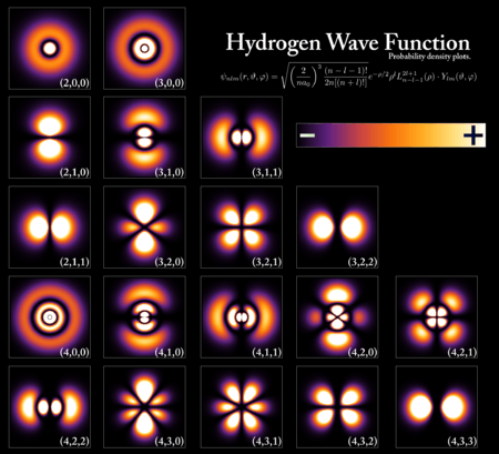
Pure states are also known as state vectors or wave functions, the latter term applying particularly when they are represented as functions of position or momentum. For example, when dealing with the energy spectrum of the electron in a hydrogen atom, the relevant state vectors are identified by the principal quantum number n, the angular momentum quantum number l, the magnetic quantum number m, and the spin z-component sz. For another example, if the spin of an electron is measured in any direction, e.g. with a Stern–Gerlach experiment, there are two possible results: up or down. The Hilbert space for the electron's spin is therefore two-dimensional, constituting a qubit. A pure state here is represented by a two-dimensional complex vector , with a length of one; that is, with


where and are the absolute values of and . A mixed state, in this case, has the structure of a matrix that is Hermitian and positive semi-definite, and has trace 1.[5] A more complicated case is given (in bra–ket notation) by the singlet state, which exemplifies quantum entanglement:


which involves superposition of joint spin states for two particles with spin 1⁄2. The singlet state satisfies the property that if the particles' spins are measured along the same direction then either the spin of the first particle is observed up and the spin of the second particle is observed down, or the first one is observed down and the second one is observed up, both possibilities occurring with equal probability.
A mixed quantum state corresponds to a probabilistic mixture of pure states; however, different distributions of pure states can generate equivalent (i.e., physically indistinguishable) mixed states. The Schrödinger–HJW theorem classifies the multitude of ways to write a given mixed state as a convex combination of pure states.[6] Before a particular measurement is performed on a quantum system, the theory gives only a probability distribution for the outcome, and the form that this distribution takes is completely determined by the quantum state and the linear operators describing the measurement. Probability distributions for different measurements exhibit tradeoffs exemplified by the uncertainty principle: a state that implies a narrow spread of possible outcomes for one experiment necessarily implies a wide spread of possible outcomes for another.
Conceptual description
Pure states
In the mathematical formulation of quantum mechanics, pure quantum states correspond to vectors in a Hilbert space, while each observable quantity (such as the energy or momentum of a particle) is associated with a mathematical operator. The operator serves as a linear function which acts on the states of the system. The eigenvalues of the operator correspond to the possible values of the observable, i.e. it is possible to observe a particle with a momentum of 1 kg⋅m/s if and only if one of the eigenvalues of the momentum operator is 1 kg⋅m/s. The corresponding eigenvector (which physicists call an eigenstate) with eigenvalue 1 kg⋅m/s would be a quantum state with a definite, well-defined value of momentum of 1 kg⋅m/s, with no quantum uncertainty. If its momentum were measured, the result is guaranteed to be 1 kg⋅m/s.
On the other hand, a system in a superposition of multiple different eigenstates does in general have quantum uncertainty for the given observable. We can represent this linear combination of eigenstates as:

The coefficient which corresponds to a particular state in the linear combination is a complex number, thus allowing interference effects between states. The coefficients are time dependent. How a quantum state changes in time is governed by the time evolution operator. The symbols and [lower-alpha 1] surrounding the are part of bra–ket notation.


Statistical mixtures of states are a different type of linear combination. A statistical mixture of states is a statistical ensemble of independent systems. Statistical mixtures represent the degree of knowledge whilst the uncertainty within quantum mechanics is fundamental. Mathematically, a statistical mixture is not a combination using complex coefficients, but rather a combination using real-valued, positive probabilities of different states . A number represents the probability of a randomly selected system being in the state . Unlike the linear combination case each system is in a definite eigenstate.[7][8]


The expectation value of an observable A is a statistical mean of measured values of the observable. It is this mean, and the distribution of probabilities, that is predicted by physical theories.

There is no state which is simultaneously an eigenstate for all observables. For example, we cannot prepare a state such that both the position measurement Q(t) and the momentum measurement P(t) (at the same time t) are known exactly; at least one of them will have a range of possible values.[lower-alpha 2] This is the content of the Heisenberg uncertainty relation.
Moreover, in contrast to classical mechanics, it is unavoidable that performing a measurement on the system generally changes its state.[9][10][lower-alpha 3] More precisely: After measuring an observable A, the system will be in an eigenstate of A; thus the state has changed, unless the system was already in that eigenstate. This expresses a kind of logical consistency: If we measure A twice in the same run of the experiment, the measurements being directly consecutive in time,[lower-alpha 4] then they will produce the same results. This has some strange consequences, however, as follows.
Consider two incompatible observables, A and B, where A corresponds to a measurement earlier in time than B.[lower-alpha 5] Suppose that the system is in an eigenstate of B at the experiment's beginning. If we measure only B, all runs of the experiment will yield the same result. If we measure first A and then B in the same run of the experiment, the system will transfer to an eigenstate of A after the first measurement, and we will generally notice that the results of B are statistical. Thus: Quantum mechanical measurements influence one another, and the order in which they are performed is important.
Another feature of quantum states becomes relevant if we consider a physical system that consists of multiple subsystems; for example, an experiment with two particles rather than one. Quantum physics allows for certain states, called entangled states, that show certain statistical correlations between measurements on the two particles which cannot be explained by classical theory. For details, see entanglement. These entangled states lead to experimentally testable properties (Bell's theorem) that allow us to distinguish between quantum theory and alternative classical (non-quantum) models.
Schrödinger picture vs. Heisenberg picture
One can take the observables to be dependent on time, while the state σ was fixed once at the beginning of the experiment. This approach is called the Heisenberg picture. (This approach was taken in the later part of the discussion above, with time-varying observables P(t), Q(t).) One can, equivalently, treat the observables as fixed, while the state of the system depends on time; that is known as the Schrödinger picture. (This approach was taken in the earlier part of the discussion above, with a time-varying state .) Conceptually (and mathematically), the two approaches are equivalent; choosing one of them is a matter of convention.

Both viewpoints are used in quantum theory. While non-relativistic quantum mechanics is usually formulated in terms of the Schrödinger picture, the Heisenberg picture is often preferred in a relativistic context, that is, for quantum field theory. Compare with Dirac picture.[12]:65
Formalism in quantum physics
Pure states as rays in a Hilbert space
Quantum physics is most commonly formulated in terms of linear algebra, as follows. Any given system is identified with some finite- or infinite-dimensional Hilbert space. The pure states correspond to vectors of norm 1. Thus the set of all pure states corresponds to the unit sphere in the Hilbert space, because the unit sphere is defined as the set of all vectors with norm 1.
Multiplying a pure state by a scalar is physically inconsequential (as long as the state is considered by itself). If one vector is obtained from the other by multiplying by a scalar of unit magnitude, the two vectors are said to correspond to the same "ray" in Hilbert space[1]:50 and also to the same point in the projective Hilbert space.
Bra–ket notation
Calculations in quantum mechanics make frequent use of linear operators, scalar products, dual spaces and Hermitian conjugation. In order to make such calculations flow smoothly, and to make it unnecessary (in some contexts) to fully understand the underlying linear algebra, Paul Dirac invented a notation to describe quantum states, known as bra–ket notation. Although the details of this are beyond the scope of this article, some consequences of this are:
- The expression used to denote a state vector (which corresponds to a pure quantum state) takes the form (where the "" can be replaced by any other symbols, letters, numbers, or even words). This can be contrasted with the usual mathematical notation, where vectors are usually lower-case latin letters, and it is clear from the context that they are indeed vectors.
- Dirac defined two kinds of vector, bra and ket, dual to each other.[lower-alpha 6]
- Each ket is uniquely associated with a so-called bra, denoted , which corresponds to the same physical quantum state. Technically, the bra is the adjoint of the ket. It is an element of the dual space, and related to the ket by the Riesz representation theorem. In a finite-dimensional space with a chosen basis, writing as a column vector, is a row vector; to obtain it just take the transpose and entry-wise complex conjugate of .
- Scalar products[lower-alpha 7][lower-alpha 8] (also called brackets) are written so as to look like a bra and ket next to each other: . (The phrase "bra-ket" is supposed to resemble "bracket".)


Spin
The angular momentum has the same dimension (M·L2·T−1) as the Planck constant and, at quantum scale, behaves as a discrete degree of freedom of a quantum system. Most particles possess a kind of intrinsic angular momentum that does not appear at all in classical mechanics and arises from Dirac's relativistic generalization of the theory. Mathematically it is described with spinors. In non-relativistic quantum mechanics the group representations of the Lie group SU(2) are used to describe this additional freedom. For a given particle, the choice of representation (and hence the range of possible values of the spin observable) is specified by a non-negative number S that, in units of Planck's reduced constant ħ, is either an integer (0, 1, 2 ...) or a half-integer (1/2, 3/2, 5/2 ...). For a massive particle with spin S, its spin quantum number m always assumes one of the 2S + 1 possible values in the set

As a consequence, the quantum state of a particle with spin is described by a vector-valued wave function with values in C2S+1. Equivalently, it is represented by a complex-valued function of four variables: one discrete quantum number variable (for the spin) is added to the usual three continuous variables (for the position in space).
Many-body states and particle statistics
The quantum state of a system of N particles, each potentially with spin, is described by a complex-valued function with four variables per particle, corresponding to 3 spatial coordinates and spin, e.g.

Here, the spin variables mν assume values from the set

where is the spin of νth particle. for a particle that does not exhibit spin.


The treatment of identical particles is very different for bosons (particles with integer spin) versus fermions (particles with half-integer spin). The above N-particle function must either be symmetrized (in the bosonic case) or anti-symmetrized (in the fermionic case) with respect to the particle numbers. If not all N particles are identical, but some of them are, then the function must be (anti)symmetrized separately over the variables corresponding to each group of identical variables, according to its statistics (bosonic or fermionic).
Electrons are fermions with S = 1/2, photons (quanta of light) are bosons with S = 1 (although in the vacuum they are massless and can't be described with Schrödinger mechanics).
When symmetrization or anti-symmetrization is unnecessary, N-particle spaces of states can be obtained simply by tensor products of one-particle spaces, to which we will return later.
Basis states of one-particle systems
As with any Hilbert space, if a basis is chosen for the Hilbert space of a system, then any ket can be expanded as a linear combination of those basis elements. Symbolically, given basis kets , any ket can be written


where ci are complex numbers. In physical terms, this is described by saying that has been expressed as a quantum superposition of the states . If the basis kets are chosen to be orthonormal (as is often the case), then .

One property worth noting is that the normalized states are characterized by

and for orthonormal basis this translates to

Expansions of this sort play an important role in measurement in quantum mechanics. In particular, if the are eigenstates (with eigenvalues ki) of an observable, and that observable is measured on the normalized state , then the probability that the result of the measurement is ki is |ci|2. (The normalization condition above mandates that the total sum of probabilities is equal to one.)
A particularly important example is the position basis, which is the basis consisting of eigenstates with eigenvalues of the observable which corresponds to measuring position.[lower-alpha 9] If these eigenstates are nondegenerate (for example, if the system is a single, spinless particle), then any ket is associated with a complex-valued function of three-dimensional space


- [lower-alpha 11] i.e. (a Dirac delta function), which means that </ref>


This function is called the wave function corresponding to . Similarly to the discrete case above, the probability density of the particle being found at position is and the normalized states have

- .

In terms of the continuous set of position basis , the state is:
- .

Superposition of pure states
As mentioned above, quantum states may be superposed. If and are two kets corresponding to quantum states, the ket


is a different quantum state (possibly not normalized). Note that both the amplitudes and phases (arguments) of and will influence the resulting quantum state. In other words, for example, even though and (for real θ) correspond to the same physical quantum state, they are not interchangeable, since and will not correspond to the same physical state for all choices of . However, and will correspond to the same physical state. This is sometimes described by saying that "global" phase factors are unphysical, but "relative" phase factors are physical and important.


One practical example of superposition is the double-slit experiment, in which superposition leads to quantum interference. The photon state is a superposition of two different states, one corresponding to the photon travel through the left slit, and the other corresponding to travel through the right slit. The relative phase of those two states depends on the difference of the distances from the two slits. Depending on that phase, the interference is constructive at some locations and destructive in others, creating the interference pattern. We may say that superposed states are in coherent superposition, by analogy with coherence in other wave phenomena.
Another example of the importance of relative phase in quantum superposition is Rabi oscillations, where the relative phase of two states varies in time due to the Schrödinger equation. The resulting superposition ends up oscillating back and forth between two different states.
Mixed states
A pure quantum state is a state which can be described by a single ket vector, as described above. A mixed quantum state is a statistical ensemble of pure states (see quantum statistical mechanics). Mixed states inevitably arise from pure states when, for a composite quantum system with an entangled state on it, the part is inaccessible to the observer. The state of the part is expressed then as the partial trace over .


A mixed state cannot be described with a single ket vector. Instead, it is described by its associated density matrix (or density operator), usually denoted ρ. Note that density matrices can describe both mixed and pure states, treating them on the same footing. Moreover, a mixed quantum state on a given quantum system described by a Hilbert space can be always represented as the partial trace of a pure quantum state (called a purification) on a larger bipartite system for a sufficiently large Hilbert space .


The density matrix describing a mixed state is defined to be an operator of the form

where is the fraction of the ensemble in each pure state The density matrix can be thought of as a way of using the one-particle formalism to describe the behavior of many similar particles by giving a probability distribution (or ensemble) of states that these particles can be found in.


A simple criterion for checking whether a density matrix is describing a pure or mixed state is that the trace of ρ2 is equal to 1 if the state is pure, and less than 1 if the state is mixed.[lower-alpha 12][13] Another, equivalent, criterion is that the von Neumann entropy is 0 for a pure state, and strictly positive for a mixed state.
The rules for measurement in quantum mechanics are particularly simple to state in terms of density matrices. For example, the ensemble average (expectation value) of a measurement corresponding to an observable A is given by

where are eigenkets and eigenvalues, respectively, for the operator A, and "tr" denotes trace. It is important to note that two types of averaging are occurring, one being a weighted quantum superposition over the basis kets of the pure states, and the other being a statistical (said incoherent) average with the probabilities ps of those states.


According to Eugene Wigner,[14] the concept of mixture was put forward by Lev Landau.[15][16]:38–41
Mathematical generalizations
States can be formulated in terms of observables, rather than as vectors in a vector space. These are positive normalized linear functionals on a C*-algebra, or sometimes other classes of algebras of observables. See State on a C*-algebra and Gelfand–Naimark–Segal construction for more details.
See also
- Atomic electron transition
- Bloch sphere
- Greenberger–Horne–Zeilinger state
- Ground state
- Introduction to quantum mechanics
- No-cloning theorem
- Orthonormal basis
- PBR theorem
- Quantum harmonic oscillator
- Quantum logic gate
- State vector reduction, for historical reasons called a wave function collapse
- Stationary state
- W state
Notes
- Sometimes written ">"; see angle brackets.
- To avoid misunderstandings: Here we mean that Q(t) and P(t) are measured in the same state, but not in the same run of the experiment.
- Dirac (1958),[11] p. 4: "If a system is small, we cannot observe it without producing a serious disturbance."
- i.e. separated by a zero delay. One can think of it as stopping the time, then making the two measurements one after the other, then resuming the time. Thus, the measurements occurred at the same time, but it is still possible to tell which was first.
- For concreteness' sake, suppose that A = Q(t1) and B = P(t2) in the above example, with t2 > t1 > 0.
- Dirac (1958),[11] p. 20: "The bra vectors, as they have been here introduced, are quite a different kind of vector from the kets, and so far there is no connexion between them except for the existence of a scalar product of a bra and a ket."
- Dirac (1958),[11] p. 19: "A scalar product 〈B|A〉 now appears as a complete bracket expression."
- Gottfried (2013),[12] p. 31: "to define the scalar products as being between bras and kets."
- Note that a state is a superposition of different basis states , so and are elements of the same Hilbert space. A particle in state is located precisely at position , while a particle in state can be found at different positions with corresponding probabilities.
- Landau (1965),<ref name='Landau (1965)' group=''>
- In the continuous case, the basis kets are not unit kets (unlike the state ): They are normalized according to [lower-alpha 10] p. 17: "∫ Ψf′Ψf* dq = δ(f′ − f)" (the left side corresponds to 〈f|f′〉), "∫ δ(f′ − f) df′ = 1".
- Note that this criterion works when the density matrix is normalized so that the trace of ρ is 1, as it is for the standard definition given in this section. Occasionally a density matrix will be normalized differently, in which case the criterion is


References
- Weinberg, S. (2002), The Quantum Theory of Fields, I, Cambridge University Press, ISBN 978-0-521-55001-7
- Griffiths, David J. (2004), Introduction to Quantum Mechanics (2nd ed.), Prentice Hall, ISBN 978-0-13-111892-8
- Holevo, Alexander S. (2001). Statistical Structure of Quantum Theory. Lecture Notes in Physics. Springer. ISBN 3-540-42082-7. OCLC 318268606.
- Peres, Asher (1995). Quantum Theory: Concepts and Methods. Kluwer Academic Publishers. ISBN 0-7923-2549-4.
- Rieffel, Eleanor G.; Polak, Wolfgang H. (2011-03-04). Quantum Computing: A Gentle Introduction. MIT Press. ISBN 978-0-262-01506-6.
- Kirkpatrick, K. A. (February 2006). "The Schrödinger-HJW Theorem". Foundations of Physics Letters. 19 (1): 95–102. arXiv:quant-ph/0305068. doi:10.1007/s10702-006-1852-1. ISSN 0894-9875.
- Statistical Mixture of States
- "The Density Matrix". Archived from the original on January 15, 2012. Retrieved January 24, 2012.
- Heisenberg, W. (1927). Über den anschaulichen Inhalt der quantentheoretischen Kinematik und Mechanik, Z. Phys. 43: 172–198. Translation as 'The actual content of quantum theoretical kinematics and mechanics'. Also translated as 'The physical content of quantum kinematics and mechanics' at pp. 62–84 by editors John Wheeler and Wojciech Zurek, in Quantum Theory and Measurement (1983), Princeton University Press, Princeton NJ.
- Bohr, N. (1927/1928). The quantum postulate and the recent development of atomic theory, Nature Supplement April 14 1928, 121: 580–590.
- Dirac, P.A.M. (1958). The Principles of Quantum Mechanics, 4th edition, Oxford University Press, Oxford UK.
- Gottfried, Kurt; Yan, Tung-Mow (2003). Quantum Mechanics: Fundamentals (2nd, illustrated ed.). Springer. ISBN 9780387955766.
- Blum, Density matrix theory and applications, page 39.
- Eugene Wigner (1962). "Remarks on the mind-body question" (PDF). In I.J. Good (ed.). The Scientist Speculates. London: Heinemann. pp. 284–302. Footnote 13 on p.180
- Lev Landau (1927). "Das Dämpfungsproblem in der Wellenmechanik (The Damping Problem in Wave Mechanics)". Zeitschrift für Physik. 45 (5–6): 430–441. Bibcode:1927ZPhy...45..430L. doi:10.1007/bf01343064. English translation reprinted in: D. Ter Haar, ed. (1965). Collected papers of L.D. Landau. Oxford: Pergamon Press. p.8–18
- Lev Landau; Evgeny Lifshitz (1965). Quantum Mechanics — Non-Relativistic Theory (PDF). Course of Theoretical Physics. 3 (2nd ed.). London: Pergamon Press.
Further reading
The concept of quantum states, in particular the content of the section Formalism in quantum physics above, is covered in most standard textbooks on quantum mechanics.
For a discussion of conceptual aspects and a comparison with classical states, see:
- Isham, Chris J (1995). Lectures on Quantum Theory: Mathematical and Structural Foundations. Imperial College Press. ISBN 978-1-86094-001-9.
For a more detailed coverage of mathematical aspects, see:
- Bratteli, Ola; Robinson, Derek W (1987). Operator Algebras and Quantum Statistical Mechanics 1. Springer. ISBN 978-3-540-17093-8. 2nd edition. In particular, see Sec. 2.3.
For a discussion of purifications of mixed quantum states, see Chapter 2 of John Preskill's lecture notes for Physics 219 at Caltech.
For a discussion of geometric aspects see:
- Bengtsson I; Życzkowski K (2006). Geometry of Quantum States. Cambridge: Cambridge University Press., second, revised edition (2017)
| Background | |||||||
|---|---|---|---|---|---|---|---|
| Fundamentals | |||||||
| Mathematics |
| ||||||
| Interpretations | |||||||
| Experiments | |||||||
| Science |
| ||||||
| Technologies | |||||||
| Extensions | |||||||
| Related | |||||||
| |||||||