Ornstein–Uhlenbeck process
In mathematics, the Ornstein–Uhlenbeck process is a stochastic process with applications in financial mathematics and the physical sciences. Its original application in physics was as a model for the velocity of a massive Brownian particle under the influence of friction. It is named after Leonard Ornstein and George Eugene Uhlenbeck.
The Ornstein–Uhlenbeck process is a stationary Gauss–Markov process, which means that it is a Gaussian process, a Markov process, and is temporally homogeneous. In fact, it is the only nontrivial process that satisfies these three conditions, up to allowing linear transformations of the space and time variables.[1] Over time, the process tends to drift towards its mean function: such a process is called mean-reverting.
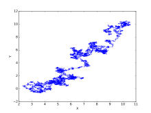
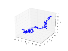
The process can be considered to be a modification of the random walk in continuous time, or Wiener process, in which the properties of the process have been changed so that there is a tendency of the walk to move back towards a central location, with a greater attraction when the process is further away from the center. The Ornstein–Uhlenbeck process can also be considered as the continuous-time analogue of the discrete-time AR(1) process.
Definition
The Ornstein–Uhlenbeck process is defined by the following stochastic differential equation:


where and are parameters and denotes the Wiener process.[2][3][4]


An additional drift term is sometimes added:

where is a constant. In financial mathematics, this is also known as the Vasicek model.[5]

The Ornstein–Uhlenbeck process is sometimes also written as a Langevin equation of the form

where , also known as white noise, stands in for the supposed derivative of the Wiener process.[6] However, does not exist because the Wiener process is nowhere differentiable, and so the Langevin equation is, strictly speaking, only heuristic.[7] In physics and engineering disciplines, it is nevertheless a common representation for the Ornstein–Uhlenbeck process and similar stochastic differential equations.


Fokker–Planck equation representation
The Ornstein–Uhlenbeck process can also be described in terms of a probability density function, , which specifies the probability of finding the process in the state at time .[8] This function satisfies the Fokker–Planck equation


where . This is a linear parabolic partial differential equation which can be solved by a variety of techniques. The transition probability is a Gaussian with mean and variance :


This gives the probability of the state occurring at time given initial state at time . Equivalently, is the solution of the Fokker-Planck equation with initial condition .


Mathematical properties
Assuming is constant, the mean is


and the covariance is

The Ornstein–Uhlenbeck process is an example of a Gaussian process that has a bounded variance and admits a stationary probability distribution, in contrast to the Wiener process; the difference between the two is in their "drift" term. For the Wiener process the drift term is constant, whereas for the Ornstein–Uhlenbeck process it is dependent on the current value of the process: if the current value of the process is less than the (long-term) mean, the drift will be positive; if the current value of the process is greater than the (long-term) mean, the drift will be negative. In other words, the mean acts as an equilibrium level for the process. This gives the process its informative name, "mean-reverting."
Properties of sample paths
A temporally homogeneous Ornstein–Uhlenbeck process can be represented as a scaled, time-transformed Wiener process:

where is the standard Wiener process.[1] Equivalently, with the change of variable this becomes


Using this mapping, one can translate known properties of into corresponding statements for . For instance, the law of the iterated logarithm for becomes[1]

Formal solution
The stochastic differential equation for can be formally solved by variation of parameters.[9] Writing

we get

Integrating from to we get


whereupon we see

From this representation, the first moment (i.e. the mean) is shown to be

assuming is constant. Moreover, the Itō isometry can be used to calculate the covariance function by

Numerical sampling
By using discretely sampled data at time intervals of width , the maximum likelihood estimators for the parameters of the Ornstein–Uhlenbeck process are asymptotically normal to their true values.[10] More precisely,

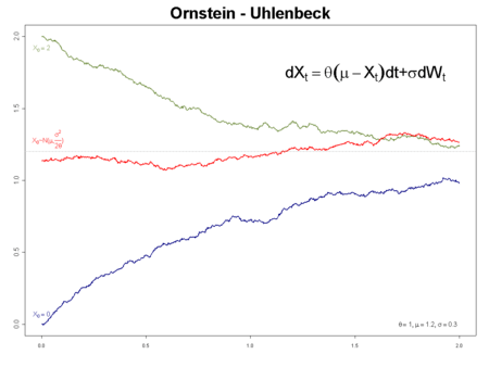
blue: initial value a = 0 (a.s.)
green: initial value a = 2 (a.s.)
red: initial value normally distributed so that the process has invariant measure
Scaling limit interpretation
The Ornstein–Uhlenbeck process can be interpreted as a scaling limit of a discrete process, in the same way that Brownian motion is a scaling limit of random walks. Consider an urn containing blue and yellow balls. At each step a ball is chosen at random and replaced by a ball of the opposite colour. Let be the number of blue balls in the urn after steps. Then converges in law to an Ornstein–Uhlenbeck process as tends to infinity.


Application in physical sciences
The Ornstein–Uhlenbeck process is a prototype of a noisy relaxation process. Consider for example a Hookean spring with spring constant whose dynamics is highly overdamped with friction coefficient . In the presence of thermal fluctuations with temperature , the length of the spring will fluctuate stochastically around the spring rest length ; its stochastic dynamic is described by an Ornstein–Uhlenbeck process with:


where is derived from the Stokes–Einstein equation for the effective diffusion constant.


In physical sciences, the stochastic differential equation of an Ornstein–Uhlenbeck process is rewritten as a Langevin equation

where is white Gaussian noise with Fluctuations are correlated as


with correlation time .

At equilibrium, the spring stores an average energy in accordance with the equipartition theorem.

Application in financial mathematics
The Ornstein–Uhlenbeck process is one of several approaches used to model (with modifications) interest rates, currency exchange rates, and commodity prices stochastically. The parameter represents the equilibrium or mean value supported by fundamentals; the degree of volatility around it caused by shocks, and the rate by which these shocks dissipate and the variable reverts towards the mean. One application of the process is a trading strategy known as pairs trade.[11][12][13]

Application in evolutionary biology
The Ornstein–Uhlenbeck process has been proposed as an improvement over a Brownian motion model for modeling the change in organismal phenotypes over time.[14] A Brownian motion model implies that the phenotype can move without limit, whereas for most phenotypes natural selection imposes a cost for moving too far in either direction.
Generalizations
It is possible to extend Ornstein–Uhlenbeck processes to processes where the background driving process is a Lévy process (instead of a simple Brownian motion). These processes are widely studied by Ole Barndorff-Nielsen and Neil Shephard, and others.
In addition, in finance, stochastic processes are used where the volatility increases for larger values of . In particular, the CKLS (Chan–Karolyi–Longstaff–Sanders) process[15] with the volatility term replaced by can be solved in closed form for , as well as for , which corresponds to the conventional OU process. Another special case is , which corresponds to the Cox–Ingersoll–Ross model (CIR-model).


Higher dimensions
A multi-dimensional version of the Ornstein–Uhlenbeck process, denoted by the N-dimensional vector , can be defined from


where is an N-dimensional Wiener process, and and are constant N×N matrices.[16] The solution is


and the mean is

Note that these expressions make use of the matrix exponential.
The process can also be described in terms of the probability density function , which satisfies the Fokker–Planck equation[17]


where the matrix with components is defined by . As for the 1d case, the process is a linear transformation of Gaussian random variables, and therefore itself must be Gaussian. Because of this, the transition probability is a Gaussian which can be written down explicitly. If the real parts of the eigenvalues of are larger than zero, a stationary solution moreover exists, given by


where the matrix is determined from .[18]


See also
- Stochastic calculus
- Wiener process
- Gaussian process
- Mathematical finance
- The Vasicek model of interest rates
- Short rate model
- Diffusion
- Fluctuation-dissipation theorem
Notes
- Doob, J.L. (April 1942). "The Brownian Movement and Stochastic Equations". Annals of Mathematics. 43 (2): 351–369. doi:10.2307/1968873. JSTOR 1968873.
- Karatzas, Ioannis; Shreve, Steven E. (1991), Brownian Motion and Stochastic Calculus (2nd ed.), Springer-Verlag, p. 358, ISBN 978-0-387-97655-6
- Gard, Thomas C. (1988), Introduction to Stochastic Differential Equations, Marcel Dekker, p. 115, ISBN 978-0-8247-7776-0
- Gardiner, C.W. (1985), Handbook of Stochastic Methods (2nd ed.), Springer-Verlag, p. 106, ISBN 978-0-387-15607-1
- Björk, Tomas (2009). Arbitrage Theory in Continuous Time (3rd ed.). Oxford University Press. pp. 375, 381. ISBN 978-0-19-957474-2.
- Risken (1984)
- Lawler, Gregory F. (2006). Introduction to Stochastic Processes (2nd ed.). Chapman & Hall/CRC. ISBN 978-1584886518.CS1 maint: ref=harv (link)
- Risken, H. (1984), The Fokker-Planck Equation: Methods of Solution and Application, Springer-Verlag, pp. 99–100, ISBN 978-0-387-13098-9
- Gardiner (1985) p. 106
- Aït-Sahalia, Y. (April 2002). "Maximum Likelihood Estimation of Discretely Sampled Diffusion: A Closed-Form Approximation Approach". Econometrica. 70 (1): 223–262. doi:10.1111/1468-0262.00274.
- Optimal Mean-Reversion Trading: Mathematical Analysis and Practical Applications. World Scientific Publishing Co. 2016. ISBN 978-9814725910.
- Advantages of Pair Trading: Market Neutrality
- An Ornstein-Uhlenbeck Framework for Pairs Trading
- Martins, E.P. (1994). "Estimating the Rate of Phenotypic Evolution from Comparative Data". Amer. Nat. 144 (2): 193–209. doi:10.1086/285670.
- Chan et al. (1992)
- Gardiner (1985), p. 109
- Gardiner (1985), p. 97
- Risken (1984), p. 156
References
- Bibbona, E.; Panfilo, G.; Tavella, P. (2008). "The Ornstein-Uhlenbeck process as a model of a low pass filtered white noise". Metrologia. 45 (6): S117–S126. Bibcode:2008Metro..45S.117B. doi:10.1088/0026-1394/45/6/S17.
- Chan, K. C.; Karolyi, G. A.; Longstaff, F. A.; Sanders, A. B. (1992). "An empirical comparison of alternative models of the short-term interest rate". Journal of Finance. 47 (3): 1209–1227. doi:10.1111/j.1540-6261.1992.tb04011.x.
- Doob, J.L. (April 1942). "The Brownian Movement and Stochastic Equations". Annals of Mathematics. 43 (2): 351–369. doi:10.2307/1968873. JSTOR 1968873.
- Gillespie, D. T. (1996). "Exact numerical simulation of the Ornstein–Uhlenbeck process and its integral". Phys. Rev. E. 54 (2): 2084–2091. Bibcode:1996PhRvE..54.2084G. doi:10.1103/PhysRevE.54.2084. PMID 9965289.
- Leung, Tim; Li, Xin (2015). "Optimal Mean Reversion Trading with Transaction Costs and Stop-Loss Exit". International Journal of Theoretical & Applied Finance. 18 (3): 1550020. arXiv:1411.5062. doi:10.1142/S021902491550020X.
- Risken, H. (1989). The Fokker–Planck Equation: Method of Solution and Applications. New York: Springer-Verlag. ISBN 978-0387504988.
- Uhlenbeck, G. E.; Ornstein, L. S. (1930). "On the theory of Brownian Motion". Phys. Rev. 36 (5): 823–841. Bibcode:1930PhRv...36..823U. doi:10.1103/PhysRev.36.823.
- Martins, E.P. (1994). "Estimating the Rate of Phenotypic Evolution from Comparative Data". Amer. Nat. 144 (2): 193–209. doi:10.1086/285670.
External links
- Review of Statistical Arbitrage, Cointegration, and Multivariate Ornstein–Uhlenbeck, Attilio Meucci
- A Stochastic Processes Toolkit for Risk Management, Damiano Brigo, Antonio Dalessandro, Matthias Neugebauer and Fares Triki
- Simulating and Calibrating the Ornstein–Uhlenbeck process, M. A. van den Berg
- Maximum likelihood estimation of mean reverting processes, Jose Carlos Garcia Franco
- "Interactive Web Application: Stochastic Processes used in Quantitative Finance". Archived from the original on 2015-09-20. Retrieved 2015-07-03.