IS–LM model
The IS–LM model, or Hicks–Hansen model, is a two-dimensional macroeconomic tool that shows the relationship between interest rates and assets market (also known as real output in goods and services market plus money market). The intersection of the "investment–saving" (IS) and "liquidity preference–money supply" (LM) curves models "general equilibrium" where supposed simultaneous equilibria occur in both the goods and the asset markets.[1] Yet two equivalent interpretations are possible: first, the IS–LM model explains changes in national income when price level is fixed short-run; second, the IS–LM model shows why an aggregate demand curve can shift.[2] Hence, this tool is sometimes used not only to analyse economic fluctuations but also to suggest potential levels for appropriate stabilisation policies.[3]
The model was developed by John Hicks in 1937,[4] and later extended by Alvin Hansen,[5] as a mathematical representation of Keynesian macroeconomic theory. Between the 1940s and mid-1970s, it was the leading framework of macroeconomic analysis.[6] While it has been largely absent from macroeconomic research ever since, it is still a backbone conceptual introductory tool in many macroeconomics textbooks.[7] By itself, the IS–LM model is used to study the short run when prices are fixed or sticky and no inflation is taken into consideration. But in practice the main role of the model is as a path to explain the AD–AS model.[2]
History
The IS–LM model was first introduced at a conference of the Econometric Society held in Oxford during September 1936. Roy Harrod, John R. Hicks, and James Meade all presented papers describing mathematical models attempting to summarize John Maynard Keynes' General Theory of Employment, Interest, and Money.[4][8] Hicks, who had seen a draft of Harrod's paper, invented the IS–LM model (originally using the abbreviation "LL", not "LM"). He later presented it in "Mr. Keynes and the Classics: A Suggested Interpretation".[4]
Although generally accepted as being imperfect, the model is seen as a useful pedagogical tool for imparting an understanding of the questions that macroeconomists today attempt to answer through more nuanced approaches. As such, it is included in most undergraduate macroeconomics textbooks, but omitted from most graduate texts due to the current dominance of real business cycle and new Keynesian theories.[9]
Formation
The point where the IS and LM schedules intersect represents a short-run equilibrium in the real and monetary sectors (though not necessarily in other sectors, such as labor markets): both the product market and the money market are in equilibrium. This equilibrium yields a unique combination of the interest rate and real GDP.
IS (investment–saving) curve
The IS curve shows the causation from interest rates to planned investment to national income and output.
For the investment–saving curve, the independent variable is the interest rate and the dependent variable is the level of income. The IS curve is drawn as downward-sloping with the interest rate r on the vertical axis and GDP (gross domestic product: Y) on the horizontal axis. The IS curve represents the locus where total spending (consumer spending + planned private investment + government purchases + net exports) equals total output (real income, Y, or GDP).
The IS curve also represents the equilibria where total private investment equals total saving, with saving equal to consumer saving plus government saving (the budget surplus) plus foreign saving (the trade surplus). The level of real GDP (Y) is determined along this line for each interest rate. Every level of the real interest rate will generate a certain level of investment and spending: lower interest rates encourage higher investment and more spending. The multiplier effect of an increase in fixed investment resulting from a lower interest rate raises real GDP. This explains the downward slope of the IS curve. In summary, the IS curve shows the causation from interest rates to planned fixed investment to rising national income and output.
The IS curve is defined by the equation

where Y represents income, represents consumer spending increasing as a function of disposable income (income, Y, minus taxes, T(Y), which themselves depend positively on income), represents business investment decreasing as a function of the real interest rate, G represents government spending, and NX(Y) represents net exports (exports minus imports) decreasing as a function of income (decreasing because imports are an increasing function of income).


LM curve
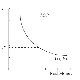
The LM curve shows the combinations of interest rates and levels of real income for which the money market is in equilibrium. It shows where money demand equals money supply. For the LM curve, the independent variable is income and the dependent variable is the interest rate.
In the money market equilibrium diagram, the liquidity preference function is the willingness to hold cash. The liquidity preference function is downward sloping (i.e. the willingness to hold cash increases as the interest rate decreases). Two basic elements determine the quantity of cash balances demanded:
- 1) Transactions demand for money: this includes both (a) the willingness to hold cash for everyday transactions and (b) a precautionary measure (money demand in case of emergencies). Transactions demand is positively related to real GDP. As GDP is considered exogenous to the liquidity preference function, changes in GDP shift the curve.
- 2) Speculative demand for money: this is the willingness to hold cash instead of securities as an asset for investment purposes. Speculative demand is inversely related to the interest rate. As the interest rate rises, the opportunity cost of holding money rather than investing in securities increases. So, as interest rates rise, speculative demand for money falls.
Money supply is determined by central bank decisions and willingness of commercial banks to loan money. Money supply in effect is perfectly inelastic with respect to nominal interest rates. Thus the money supply function is represented as a vertical line – money supply is a constant, independent of the interest rate, GDP, and other factors. Mathematically, the LM curve is defined by the equation , where the supply of money is represented as the real amount M/P (as opposed to the nominal amount M), with P representing the price level, and L being the real demand for money, which is some function of the interest rate and the level of real income.

An increase in GDP shifts the liquidity preference function rightward and hence increases the interest rate. Thus the LM function is positively sloped.
Shifts
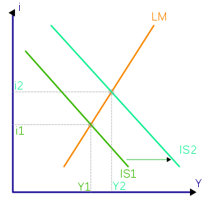
One hypothesis is that a government's deficit spending ("fiscal policy") has an effect similar to that of a lower saving rate or increased private fixed investment, increasing the amount of demand for goods at each individual interest rate. An increased deficit by the national government shifts the IS curve to the right. This raises the equilibrium interest rate (from i1 to i2) and national income (from Y1 to Y2), as shown in the graph above. The equilibrium level of national income in the IS–LM diagram is referred to as aggregate demand.
Keynesians argue spending may actually "crowd in" (encourage) private fixed investment via the accelerator effect, which helps long-term growth. Further, if government deficits are spent on productive public investment (e.g., infrastructure or public health) that spending directly and eventually raises potential output, although not necessarily more (or less) than the lost private investment might have. The extent of any crowding out depends on the shape of the LM curve. A shift in the IS curve along a relatively flat LM curve can increase output substantially with little change in the interest rate. On the other hand, an rightward shift in the IS curve along a vertical LM curve will lead to higher interest rates, but no change in output (this case represents the "Treasury view").
Rightward shifts of the IS curve also result from exogenous increases in investment spending (i.e., for reasons other than interest rates or income), in consumer spending, and in export spending by people outside the economy being modelled, as well as by exogenous decreases in spending on imports. Thus these too raise both equilibrium income and the equilibrium interest rate. Of course, changes in these variables in the opposite direction shift the IS curve in the opposite direction.
The IS–LM model also allows for the role of monetary policy. If the money supply is increased, that shifts the LM curve downward or to the right, lowering interest rates and raising equilibrium national income. Further, exogenous decreases in liquidity preference, perhaps due to improved transactions technologies, lead to downward shifts of the LM curve and thus increases in income and decreases in interest rates. Changes in these variables in the opposite direction shift the LM curve in the opposite direction.
Incorporation into larger models
By itself, the IS–LM model is used to study the short run when prices are fixed or sticky and no inflation is taken into consideration. But in practice the main role of the model is as a sub-model of larger models (especially the Aggregate Demand-Aggregate Supply model – the AD–AS model) which allow for a flexible price level. In the aggregate demand-aggregate supply model, each point on the aggregate demand curve is an outcome of the IS–LM model for aggregate demand Y based on a particular price level. Starting from one point on the aggregate demand curve, at a particular price level and a quantity of aggregate demand implied by the IS–LM model for that price level, if one considers a higher potential price level, in the IS–LM model the real money supply M/P will be lower and hence the LM curve will be shifted higher, leading to lower aggregate demand as measured by the horizontal location of the IS–LM intersection; hence at the higher price level the level of aggregate demand is lower, so the aggregate demand curve is negatively sloped.
See also
- Keynesian cross
- AD–IA model
- IS/MP model
- Mundell–Fleming model
- National savings
- Policy mix
References
- Gordon, Robert J. (2009). Macroeconomics (Eleventh ed.). Boston: Pearson Addison Wesley. ISBN 9780321552075.
- Mankiw, N. Gregory (2012). Macroeconomics (Eighth ed.). New York: Worth Publishers. ISBN 9781429240024.
- Sloman, John; Wride, Alison (2009). Economics (Seventh ed.). Prentice Hall. ISBN 9780273715627.
- Hicks, J. R. (1937). "Mr. Keynes and the 'Classics': A Suggested Interpretation". Econometrica. 5 (2): 147–159. doi:10.2307/1907242. JSTOR 1907242.
- Hansen, A. H. (1953). A Guide to Keynes. New York: McGraw Hill.
- Bentolila, Samuel (2005). "Hicks–Hansen model". An Eponymous Dictionary of Economics: A Guide to Laws and Theorems Named after Economists. Edward Elgar. ISBN 978-1-84376-029-0.
- Colander, David (2004). "The Strange Persistence of the IS-LM Model" (PDF). History of Political Economy. 36 (Annual Supplement): 305–322. CiteSeerX 10.1.1.692.6446. doi:10.1215/00182702-36-suppl_1-305.
- Meade, J. E. (1937). "A Simplified Model of Mr. Keynes' System". Review of Economic Studies. 4 (2): 98–107. doi:10.2307/2967607. JSTOR 2967607.
- Mankiw, N. Gregory (May 2006). "The Macroeconomist as Scientist and Engineer" (PDF). p. 19. Retrieved 2014-11-17.
Further reading
- Ackley, Gardner (1978). "The 'IS–LM' Form of the Model". Macroeconomics: Theory and Policy. New York: Macmillan. pp. 358–383. ISBN 978-0-02-300290-8.
- Barro, Robert J. (1984). "The Keynesian Theory of Business Fluctuations". Macroeconomics. New York: John Wiley. pp. 487–513. ISBN 978-0-471-87407-2.
- Darby, Michael R. (1976). "The Complete Keynesian Model". Macroeconomics. New York: McGraw-Hill. pp. 285–304. ISBN 978-0-07-015346-2.
- Dernburg, Thomas F.; McDougall, Duncan M. (1980). "Macroeconomic Equilibrium: The Level of Economic Activity". Macroeconomics (Sixth ed.). New York: McGraw-Hill. pp. 53–229. ISBN 978-0-07-016534-2.
- Keiser, Norman F. (1975). "The Real-Goods and Monetary Spheres". Macroeconomics (Second ed.). New York: Random House. pp. 231–260. ISBN 978-0-394-31922-3.
- Leijonhufvud, Axel (1983). "What is Wrong with IS/LM?". In Fitoussi, Jean-Paul (ed.). Modern Macroeconomic Theory. Oxford: Blackwell. pp. 49–90. ISBN 978-0-631-13158-8.
- Mankiw, N. Gregory (2013). "Aggregate Demand I+II". Macroeconomics (Eighth international ed.). London: Palgrave Macmillan. pp. 301–352. ISBN 978-1-4641-2167-8.
- Sawyer, John A. (1989). "A Model from Keynes's General Theory". Macroeconomic Theory. New York: Harvester Wheatsheaf. pp. 62–95. ISBN 978-0-7450-0555-3.
- Smith, Warren L. (1956). "A Graphical Exposition of the Complete Keynesian System". Southern Economic Journal. 23 (2): 115–125. doi:10.2307/1053551. JSTOR 1053551.
- Vroey, Michel de; Hoover, Kevin D., eds. (2004). The IS-LM model: Its Rise, Fall, and Strange Persistence. Durham: Duke University Press. ISBN 978-0-8223-6631-7.
- Young, Warren; Zilberfarb, Ben-Zion, eds. (2000). IS-LM and Modern Macroeconomics. Recent Economic Thought. 73. Springer Science & Business Media. ISBN 978-0-7923-7966-9.
External links
| Wikiquote has quotations related to: IS–LM model |
| Wikimedia Commons has media related to IS-LM model diagrams. |
- Krugman, Paul. There's something about macro – An explanation of the model and its role in understanding macroeconomics.
- Krugman, Paul. IS-LMentary – A basic explanation of the model and its uses.
- Wiens, Elmer G. IS–LM model – An online, interactive IS–LM model of the Canadian economy.