Supply and demand
In microeconomics, supply and demand is an economic model of price determination in a market. It postulates that, holding all else equal, in a competitive market, the unit price for a particular good, or other traded item such as labor or liquid financial assets, will vary until it settles at a point where the quantity demanded (at the current price) will equal the quantity supplied (at the current price), resulting in an economic equilibrium for price and quantity transacted.
| Part of a series on |
| Economics |
|---|
|
|
|
By application |
|
Notable economists |
|
Lists |
|
Glossary |
|
Graphical representations
Although it is normal to regard the quantity demanded and the quantity supplied as functions of the price of the goods, the standard graphical representation, usually attributed to Alfred Marshall, has price on the vertical axis and quantity on the horizontal axis.
Since determinants of supply and demand other than the price of the goods in question are not explicitly represented in the diagram, changes in the values of these variables are represented by moving the supply and demand curves ("shifts" in the curves). In contrast, responses to changes in the price of the good are represented as movements along unchanged supply and demand curves.
Supply schedule
A supply schedule, depicted graphically as a supply curve, is a table that shows the relationship between the price of a good and the quantity supplied by producers. Under the assumption of perfect competition, supply is determined by marginal cost: firms will produce additional output as long as the cost of producing an extra unit is less than the market price they receive.
A hike in the cost of raw goods would decrease supply, shifting the supply curve up, while a production cost discount would increase supply, shifting costs down and hurting producers as producer surplus decreases.
Mathematically, a supply curve is represented by a supply function, giving the quantity supplied as a function of its price and as many other variables as desired to better explain quantity supplied. The two most common specifications are linear supply, e.g., the slanted line

and the constant-elasticity supply function (also called isoelastic or log-log or loglinear supply function), e.g., the smooth curve

which can be rewritten as

Note that really a supply curve should be drawn with price on the horizontal x-axis, since it is the independent variable. Instead, price is put on the vertical, f(x) y-axis as a matter of unfortunate historical convention.
By its very nature, the concept of a supply curve assumes that firms are perfect competitors, having no influence over the market price. This is because each point on the supply curve answers the question, "If this firm is faced with this potential price, how much output will it sell?" If a firm has market power--in violation of the perfect competitor model--its decision on how much output to bring to market influences the market price. Thus the firm is not "faced with" any given price, and a more complicated model, e.g., a monopoly or oligopoly or differentiated-product model, should be used.
Economists distinguish between the supply curve of an individual firm and the market supply curve. The market supply curve shows the total quantity supplied by all firms, so it is the sum of the quantities supplied by all suppliers at each potential price (that is, the individual firms' supply curves are added horizontally).
Economists distinguish between short-run and long-run supply curve Short run refers to a time period during which one or more inputs are fixed (typically physical capital), and the number of firms in the industry is also fixed (if it a market supply curve). long run refers to a time period during which new firms enter or existing firms exit and all inputs can be adjusted fully to any price change. Long-run supply curves are flatter than short-run counterparts (with quantity more sensitive to price, more elastic supply).
Common determinants of supply are:
- Prices of inputs, including wages
- The technology used, Productivity
- Firms' expectations about future prices
- Number of suppliers (for a market supply curve)
Demand schedule
A demand schedule, depicted graphically as a demand curve, represents the amount of a certain good that buyers are willing and able to purchase at various prices, assuming all other determinants of demand are held constant, such as income, tastes and preferences, and the prices of substitute and complementary goods. According to the law of demand, the demand curve is always downward-sloping, meaning that as the price decreases, consumers will buy more of the good.
Mathematically, a demand curve is represented by a demand function, giving the quantity demanded as a function of its price and as many other variables as desired to better explain quantity demanded. The two most common specifications are linear demand, e.g., the slanted line

and the constant-elasticity demand function (also called isoelastic or log-log or loglinear demand function), e.g., the smooth curve

which can be rewritten as

Note that really a demand curve should be drawn with price on the horizontal x-axis, since it is the indepenent variable. Instead, price is put on the vertical, f(x) y-axis as a matter of unfortunate historical convention.
Just as the supply curve parallels the marginal cost curve, the demand curve parallels marginal utility, measured in dollars.[1] Consumers will be willing to buy a given quantity of a good, at a given price, if the marginal utility of additional consumption is equal to the opportunity cost determined by the price, that is, the marginal utility of alternative consumption choices. The demand schedule is defined as the willingness and ability of a consumer to purchase a given product at a certain time.
The demand curve is generally downward-sloping, but for some goods it is upward-sloping. Two such types of goods have been given definitions and names that are in common use: Veblen goods, goods which because of fashion or signalling are more attractive at higher prices, and Giffen goods, which, by virtue of being inferior goods that absorb a large part of a consumer's income (e.g., staples such as the classic example of potatoes in Ireland), may see an increase in quantity demanded when the price rises. The reason the law of demand is violated for Giffen goods is that the rise in the price of the good has a strong income effect, sharply reducing the purchasing power of the consumer so that he switches away from luxury goods to the Giffen good, e.g., when the price of potatoes rises, the Irish peasant can no longer afford meat and eats more potatoes to cover for the lost calories.
As with the supply curve, by its very nature the concept of a demand curve requires that the purchaser be a perfect competitor—that is, that the purchaser have no influence over the market price. This is true because each point on the demand curve answers the question, "If buyers are faced with this potential price, how much of the product will they purchase?" But, if a buyer has market power (that is, the amount he buys influences the price), he is not "faced with" any given price, and we must use a more complicated model, of monopsony.
As with supply curves, economists distinguish between the demand curve for an individual and the demand curve for a market. The market demand curve is obtained by adding the quantities from the individual demand curves at each price.
Common determinants of demand are:
- Income
- Tastes and preferences
- Prices of related goods and services
- Consumers' expectations about future prices and incomes
- Number of potential consumers
- Advertising
Microeconomics
Equilibrium
Generally speaking, an equilibrium is defined to be the price-quantity pair where the quantity demanded is equal to the quantity supplied. It is represented by the intersection of the demand and supply curves.[2] The analysis of various equilibria is a fundamental aspect of microeconomics:
Market equilibrium: A situation in a market when the price is such that the quantity demanded by consumers is correctly balanced by the quantity that firms wish to supply. In this situation, the market clears.[3]
Changes in market equilibrium: Practical uses of supply and demand analysis often center on the different variables that change equilibrium price and quantity, represented as shifts in the respective curves. Comparative statics of such a shift traces the effects from the initial equilibrium to the new equilibrium.
Demand curve shifts:
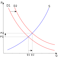
When consumers increase the quantity demanded at a given price, it is referred to as an increase in demand. Increased demand can be represented on the graph as the curve being shifted to the right. At each price point, a greater quantity is demanded, as from the initial curve D1 to the new curve D2. In the diagram, this raises the equilibrium price from P1 to the higher P2. This raises the equilibrium quantity from Q1 to the higher Q2. (A movement along the curve is described as a "change in the quantity demanded" to distinguish it from a "change in demand," that is, a shift of the curve.) The increase in demand has caused an increase in (equilibrium) quantity. The increase in demand could come from changing tastes and fashions, incomes, price changes in complementary and substitute goods, market expectations, and number of buyers. This would cause the entire demand curve to shift changing the equilibrium price and quantity. Note in the diagram that the shift of the demand curve, by causing a new equilibrium price to emerge, resulted in movement along the supply curve from the point (Q1, P1) to the point (Q2, P2).
If the demand decreases, then the opposite happens: a shift of the curve to the left. If the demand starts at D2, and decreases to D1, the equilibrium price will decrease, and the equilibrium quantity will also decrease. The quantity supplied at each price is the same as before the demand shift, reflecting the fact that the supply curve has not shifted; but the equilibrium quantity and price are different as a result of the change (shift) in demand.
Supply curve shifts:
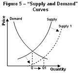
When technological progress occurs, the supply curve shifts. For example, assume that someone invents a better way of growing wheat so that the cost of growing a given quantity of wheat decreases. Otherwise stated, producers will be willing to supply more wheat at every price and this shifts the supply curve S1 outward, to S2—an increase in supply. This increase in supply causes the equilibrium price to decrease from P1 to P2. The equilibrium quantity increases from Q1 to Q2 as consumers move along the demand curve to the new lower price. As a result of a supply curve shift, the price and the quantity move in opposite directions. If the quantity supplied decreases, the opposite happens. If the supply curve starts at S2, and shifts leftward to S1, the equilibrium price will increase and the equilibrium quantity will decrease as consumers move along the demand curve to the new higher price and associated lower quantity demanded. The quantity demanded at each price is the same as before the supply shift, reflecting the fact that the demand curve has not shifted. But due to the change (shift) in supply, the equilibrium quantity and price have changed.
The movement of the supply curve in response to a change in a non-price determinant of supply is caused by a change in the y-intercept, the constant term of the supply equation. The supply curve shifts up and down the y axis as non-price determinants of demand change.
Partial equilibrium
Partial equilibrium, as the name suggests, takes into consideration only a part of the market to attain equilibrium.
Jain proposes (attributed to George Stigler): "A partial equilibrium is one which is based on only a restricted range of data, a standard example is price of a single product, the prices of all other products being held fixed during the analysis."[4]
The supply-and-demand model is a partial equilibrium model of economic equilibrium, where the clearance on the market of some specific goods is obtained independently from prices and quantities in other markets. In other words, the prices of all substitutes and complements, as well as income levels of consumers are constant. This makes analysis much simpler than in a general equilibrium model which includes an entire economy.
Here the dynamic process is that prices adjust until supply equals demand. It is a powerfully simple technique that allows one to study equilibrium, efficiency and comparative statics. The stringency of the simplifying assumptions inherent in this approach makes the model considerably more tractable, but may produce results which, while seemingly precise, do not effectively model real world economic phenomena.
Partial equilibrium analysis examines the effects of policy action in creating equilibrium only in that particular sector or market which is directly affected, ignoring its effect in any other market or industry assuming that they being small will have little impact if any.
Hence this analysis is considered to be useful in constricted markets.
Léon Walras first formalized the idea of a one-period economic equilibrium of the general economic system, but it was French economist Antoine Augustin Cournot and English political economist Alfred Marshall who developed tractable models to analyze an economic system.
Other markets
The model of supply and demand also applies to various specialty markets.
The model is commonly applied to wages, in the market for labor. The typical roles of supplier and demander are reversed. The suppliers are individuals, who try to sell their labor for the highest price. The demanders of labor are businesses, which try to buy the type of labor they need at the lowest price. The equilibrium price for a certain type of labor is the wage rate.[5] However, economist Steve Fleetwood revisited the empirical reality of supply and demand curves in labor markets and concluded that the evidence is "at best inconclusive and at worst casts doubt on their existence." For instance, he cites Kaufman and Hotchkiss (2006): "For adult men, nearly all studies find the labour supply curve to be negatively sloped or backward bending." [6]
In both classical and Keynesian economics, the money market is analyzed as a supply-and-demand system with interest rates being the price. The money supply may be a vertical supply curve, if the central bank of a country chooses to use monetary policy to fix its value regardless of the interest rate; in this case the money supply is totally inelastic. On the other hand,[7] the money supply curve is a horizontal line if the central bank is targeting a fixed interest rate and ignoring the value of the money supply; in this case the money supply curve is perfectly elastic. The demand for money intersects with the money supply to determine the interest rate.[8]
Empirical estimation
Demand and supply relations in a market can be statistically estimated from price, quantity, and other data with sufficient information in the model. This can be done with simultaneous-equation methods of estimation in econometrics. Such methods allow solving for the model-relevant "structural coefficients," the estimated algebraic counterparts of the theory. The Parameter identification problem is a common issue in "structural estimation." Typically, data on exogenous variables (that is, variables other than price and quantity, both of which are endogenous variables) are needed to perform such an estimation. An alternative to "structural estimation" is reduced-form estimation, which regresses each of the endogenous variables on the respective exogenous variables.
Macroeconomic uses
Demand and supply have also been generalized to explain macroeconomic variables in a market economy, including the quantity of total output and the general price level. The aggregate demand-aggregate supply model may be the most direct application of supply and demand to macroeconomics, but other macroeconomic models also use supply and demand. Compared to microeconomic uses of demand and supply, different (and more controversial) theoretical considerations apply to such macroeconomic counterparts as aggregate demand and aggregate supply. Demand and supply are also used in macroeconomic theory to relate money supply and money demand to interest rates, and to relate labor supply and labor demand to wage rates.
History
The 256th couplet of Tirukkural, which was composed at least 2000 years ago, says that "if people do not consume a product or service, then there will not be anybody to supply that product or service for the sake of price".[9]
According to Hamid S. Hosseini, the power of supply and demand was understood to some extent by several early Muslim scholars, such as fourteenth-century Syrian scholar Ibn Taymiyyah, who wrote: "If desire for goods increases while its availability decreases, its price rises. On the other hand, if availability of the good increases and the desire for it decreases, the price comes down."[10]
If desire for goods increases while its availability decreases, its price rises. On the other hand, if availability of the good increases and the desire for it decreases, the price comes down.

John Locke's 1691 work Some Considerations on the Consequences of the Lowering of Interest and the Raising of the Value of Money.[11] includes an early and clear description of supply and demand and their relationship. In this description demand is rent: “The price of any commodity rises or falls by the proportion of the number of buyer and sellers” and “that which regulates the price... [of goods] is nothing else but their quantity in proportion to their rent.”
The phrase "supply and demand" was first used by James Denham-Steuart in his Inquiry into the Principles of Political Economy, published in 1767. Adam Smith used the phrase in his 1776 book The Wealth of Nations, and David Ricardo titled one chapter of his 1817 work Principles of Political Economy and Taxation "On the Influence of Demand and Supply on Price".[12] Thomas Robert Malthus used the phrase "supply and demand" twenty times in the second edition of the Essay on Population in 1803.[13]
In The Wealth of Nations, Smith generally assumed that the supply price was fixed but that its "merit" (value) would decrease as its "scarcity" increased, in effect what was later called the law of demand also. Ricardo, in Principles of Political Economy and Taxation, more rigorously laid down the idea of the assumptions that were used to build his ideas of supply and demand. Antoine Augustin Cournot first developed a mathematical model of supply and demand in his 1838 Researches into the Mathematical Principles of Wealth, including diagrams.
During the late 19th century the marginalist school of thought emerged. The main innovators of this approach where Stanley Jevons, Carl Menger, and Léon Walras. The key idea was that the price was set by the subjective value of a good at the margin. This was a substantial change from Adam Smith's thoughts on determining the supply price.
In his 1870 essay "On the Graphical Representation of Supply and Demand", Fleeming Jenkin in the course of "introduc[ing] the diagrammatic method into the English economic literature" published the first drawing of supply and demand curves in English,[14] including comparative statics from a shift of supply or demand and application to the labor market.[15] The model was further developed and popularized by Alfred Marshall in the 1890 textbook Principles of Economics.[12]
Artificial intelligent buying platforms
Much of the buying and selling are now conducted online using platforms such as Amazon and eBay, where the profiles of the customers are captured and analyzed. Tshilidzi Marwala and Evan Hurwitz in their book [16] observed that the advent of artificial intelligence and related technologies such as flexible manufacturing offers the opportunity for individualized demand and supply curves to be generated. This has been found to reduce the degree of arbitrage in the market, allow for individualized pricing for the same product and brings fairness and efficiency into the market.
Criticism
The philosopher Hans Albert has argued that the ceteris paribus conditions of the marginalist theory rendered the theory itself an empty tautology and completely closed to experimental testing.[17] In essence, he argues, the supply and demand curves (theoretical functions which express the quantity of a product which would be offered or requested for a given price) are purely ontological.
Cambridge economist Joan Robinson attacked the theory in similar line, arguing that the concept is circular: "Utility is the quality in commodities that makes individuals want to buy them, and the fact that individuals want to buy commodities shows that they have utility"[18]:48 Robinson also pointed out that if we take changes in peoples' behavior in relation to a change in prices or a change in the underlying budget constraint, then we can never be sure to what extent the change in behavior was due to the change in price or budget constraint and how much was due to a change in preferences.[19]
Piero Sraffa's critique focused on the inconsistency (except in implausible circumstances) of partial equilibrium analysis and the rationale for the upward slope of the supply curve in a market for a produced consumption good.[20] The notability of Sraffa's critique is also demonstrated by Paul Samuelson's comments and engagements with it over many years, for example:
- What a cleaned-up version of Sraffa (1926) establishes is how nearly empty are all of Marshall's partial equilibrium boxes. To a logical purist of Wittgenstein and Sraffa class, the Marshallian partial equilibrium box of constant cost is even more empty than the box of increasing cost.[21]
Some economists criticize the conventional supply and demand theory for failing to explain or anticipate asset bubbles that can arise from a positive feedback loop.[22] Conventional supply and demand theory assumes that expectations of consumers do not change as a consequence of price changes. In scenarios such as the United States housing bubble, an initial price change of an asset can increase the expectations of investors, making the asset more lucrative and contributing to further price increases until market sentiment changes, which creates a positive feedback loop and an asset bubble.[23] Asset bubbles cannot be understood in the conventional supply and demand framework because the conventional system assumes a price change will be self-correcting and the system will snap back to equilibrium.
See also
- Capacity utilization
- Consumer theory
- Deadweight loss
- Economic surplus
- Effective demand
- Effect of taxes and subsidies on price
- Elasticity
- Excess demand function
- Externality
- History of economic thought
- Inverse demand function
- Law of supply
- Neoclassical economics
- Price discovery
- Rationing
- Social cost
- Supply shock
- Yield management
References
- "Marginal Utility and Demand". Retrieved 2007-02-09.
- "Microeconomics – Supply and Demand". Retrieved 2014-12-31.
- Mankiw, N.G.; Taylor, M.P. (2011). Economics (2nd ed., revised ed.). Andover: Cengage Learning.
- Jain, T.R. (2006–2007). Microeconomics and Basic Mathematics. New Delhi: VK Publications. p. 28. ISBN 978-81-87140-89-4.
- Kibbe, Matthew B. "The Minimum Wage: Washington's Perennial Myth". Cato Institute. Retrieved 2007-02-09.
- Fleetwood, Steve (August 2014). "Do labour supply and demand curves exist?". Cambridge Journal of Economics. 38 (5): 1087–113. doi:10.1093/cje/beu003.
- Basij J. Moore, Horizontalists and Verticalists: The Macroeconomics of Credit Money, Cambridge University Press, 1988
- Ritter, Lawrence S.; Silber, William L.; Udell, Gregory F. (2000). Principles of Money, Banking, and Financial Markets (10th ed.). Addison-Wesley, Menlo Park C. pp. 431–38, 465–76. ISBN 978-0-321-37557-5.
- C Chendroyaperumal (2010). The First Laws in Economics and Indian Economic Thought – Thirukkural
- Hosseini, Hamid S. (2003). "Contributions of Medieval Muslim Scholars to the History of Economics and their Impact: A Refutation of the Schumpeterian Great Gap". In Biddle, Jeff E.; Davis, Jon B.; Samuels, Warren J. (eds.). A Companion to the History of Economic Thought. Malden, MA: Blackwell. pp. 28–45 [28 & 38]. doi:10.1002/9780470999059.ch3. ISBN 978-0-631-22573-7. (citing Hamid S. Hosseini, 1995. "Understanding the Market Mechanism Before Adam Smith: Economic Thought in Medieval Islam," History of Political Economy, Vol. 27, No. 3, 539–61).
- John Locke (1691) Some Considerations on the consequences of the Lowering of Interest and the Raising of the Value of Money
- Humphrey, Thomas M. (1992). "Marshallian Cross Diagrams and their Uses before Alfred Marshall" (PDF). Economic Review (Mar/Apr): 3–23. Retrieved 2019-07-27.
- Groenewegen P. (2008) ‘Supply and Demand’. In: Palgrave Macmillan (eds) The New Palgrave Dictionary of Economics. Palgrave Macmillan, London
- A.D. Brownlie and M. F. Lloyd Prichard, 1963. "Professor Fleeming Jenkin, 1833–1885 Pioneer in Engineering and Political Economy," Oxford Economic Papers, NS, 15(3), p. 211.
- Fleeming Jenkin, 1870. "The Graphical Representation of the Laws of Supply and Demand, and their Application to Labour," in Alexander Grant, ed., (Scroll to chapter) Recess Studies, ch. VI, pp. 151–85. Edinburgh: Edmonston and Douglas
- Marwala, Tshilidzi; Hurwitz, Evan (2017). Artificial Intelligence and Economic Theory: Skynet in the Market. London: Springer. ISBN 978-3-319-66104-9.
- Fixing the Economists. 27 February 2014. Available at: Hans Albert Expands Robinson’s Critique of Marginal Utility Theory to the Law of Demand
- Robinson, Joan (1962). Economic Philosophy. Harmondsworth, Middlesex, UK: Penguin Books.
- Pilkington, Philip. Fixing the Economists. 17 February 2014. Available at: Joan Robinson's Critique of Marginal Utility Theory
- Avi J. Cohen, "'The Laws of Returns Under Competitive Conditions': Progress in Microeconomics Since Sraffa (1926)?", Eastern Economic Journal, V. 9, N. 3 (Jul.-Sep.): 1983)
- Paul A. Samuelson, "Reply" in Critical Essays on Piero Sraffa's Legacy in Economics (edited by H. D. Kurz) Cambridge University Press, 2000
- What Every Economics Student Needs to Know and Doesn't Get in the Usual Principles Text. Routledge. 2014. pp. 55, 66, 244.
- "Positive Feedback". Investopedia. Retrieved November 13, 2018.
Further reading
- Foundations of Economic Analysis by Paul A. Samuelson
- Price Theory and Applications by Steven E. Landsburg ISBN 0-538-88206-9
- An Inquiry into the Nature and Causes of the Wealth of Nations, Adam Smith, 1776
- Supply and Demand book by Hubert D. Henderson at Project Gutenberg.
External links
| Wikimedia Commons has media related to Supply and demand curves. |
| Look up supply or demand in Wiktionary, the free dictionary. |
- Nobel Prize Winner Prof. William Vickrey: 15 fatal fallacies of financial fundamentalism – A Disquisition on Demand Side Economics (William Vickrey)
- Marshallian Cross Diagrams and Their Uses before Alfred Marshall: The Origins of Supply and Demand Geometry by Thomas M. Humphrey
- By what is the price of a commodity determined?, a brief statement of Karl Marx's rival account
- Supply and Demand by Fiona Maclachlan and Basic Supply and Demand by Mark Gillis, Wolfram Demonstrations Project.