120-cell
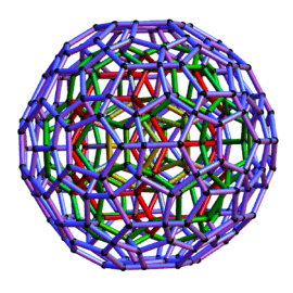
In geometry, the 120-cell is the convex regular 4-polytope with Schläfli symbol {5,3,3}. It is also called a C120, dodecaplex (short for "dodecahedral complex"), hyperdodecahedron, polydodecahedron, hecatonicosachoron, dodecacontachoron[1] and hecatonicosahedroid.[2]
| 120-cell | |
|---|---|
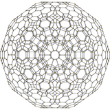
 Schlegel diagram (vertices and edges) | |
| Type | Convex regular 4-polytope |
| Schläfli symbol | {5,3,3} |
| Coxeter diagram | |
| Cells | 120 {5,3} |
| Faces | 720 {5} |
| Edges | 1200 |
| Vertices | 600 |
| Vertex figure |  tetrahedron |
| Petrie polygon | 30-gon |
| Coxeter group | H4, [3,3,5] |
| Dual | 600-cell |
| Properties | convex, isogonal, isotoxal, isohedral |
| Uniform index | 32 |
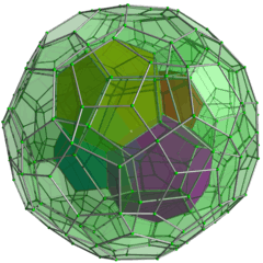
The boundary of the 120-cell is composed of 120 dodecahedral cells with 4 meeting at each vertex. It can be thought of as the 4-dimensional analog of the regular dodecahedron. Just as a dodecahedron can be built up as a model with 12 pentagons, 3 around each vertex, the dodecaplex can be built up from 120 dodecahedra, with 3 around each edge.
The Davis 120-cell, introduced by Davis (1985), is a compact 4-dimensional hyperbolic manifold obtained by identifying opposite faces of the 120-cell, whose universal cover gives the regular honeycomb {5,3,3,5} of 4-dimensional hyperbolic space.
Elements
- There are 120 cells, 720 pentagonal faces, 1200 edges, and 600 vertices.
- There are 4 dodecahedra, 6 pentagons, and 4 edges meeting at every vertex.
- There are 3 dodecahedra and 3 pentagons meeting every edge.
- The dual polytope of the 120-cell is the 600-cell.
- The compound formed from the 120-cell and its dual is the compound of 120-cell and 600-cell.
- The vertex figure of the 120-cell is a tetrahedron.
- The dihedral angle (angle between facet hyperplanes) of the 120-cell is 144°[3]
As a configuration
This configuration matrix represents the 120-cell. The rows and columns correspond to vertices, edges, faces, and cells. The diagonal numbers say how many of each element occur in the whole 120-cell. The nondiagonal numbers say how many of the column's element occur in or at the row's element.[4][5]

Here is the configuration expanded with k-face elements and k-figures. The diagonal element counts are the ratio of the full Coxeter group order, 14400, divided by the order of the subgroup with mirror removal.
| H4 | k-face | fk | f0 | f1 | f2 | f3 | k-fig | Notes | |
|---|---|---|---|---|---|---|---|---|---|
| A3 | ( ) | f0 | 600 | 4 | 6 | 4 | {3,3} | H4/A3 = 14400/24 = 600 | |
| A1A2 | { } | f1 | 2 | 720 | 3 | 3 | {3} | H4/A2A1 = 14400/6/2 = 1200 | |
| H2A1 | {5} | f2 | 5 | 5 | 1200 | 2 | { } | H4/H2A1 = 14400/10/2 = 720 | |
| H3 | {5,3} | f3 | 20 | 30 | 12 | 120 | ( ) | H4/H3 = 14400/120 = 120 |
Cartesian coordinates
The 600 vertices of a 120-cell with an edge length of 2/φ2 = 3−√5 and a center-to-vertex radius of √8 = 2 √2 include all permutations of:[6]
- (0, 0, ±2, ±2)
- (±1, ±1, ±1, ±√5)
- (±φ−2, ±φ, ±φ, ±φ)
- (±φ−1, ±φ−1, ±φ−1, ±φ2)
and all even permutations of
- (0, ±φ−2, ±1, ±φ2)
- (0, ±φ−1, ±φ, ±√5)
- (±φ−1, ±1, ±φ, ±2)
where φ (also called τ) is the golden ratio, 1 + √5/2.
Considering the adjacency matrix of the vertices representing its polyhedral graph, the graph diameter is 15, connecting each vertex to its coordinate-negation, at a Euclidean distance of 4√2 away (its circumdiameter), and there are 24 different paths to connect them along the polytope edges. From each vertex, there are 4 vertices at distance 1, 12 at distance 2, 24 at distance 3, 36 at distance 4, 52 at distance 5, 68 at distance 6, 76 at distance 7, 78 at distance 8, 72 at distance 9, 64 at distance 10, 56 at distance 11, 40 at distance 12, 12 at distance 13, 4 at distance 14, and 1 at distance 15. The adjacency matrix has 27 distinct eigenvalues ranging from 2−3φ, with a multiplicity of 4, to 4, with a multiplicity of 1. The multiplicity of eigenvalue 0 is 18, and the rank of the adjacency matrix is 582.
Visualization
The 120-cell consists of 120 dodecahedral cells. For visualization purposes, it is convenient that the dodecahedron has opposing parallel faces (a trait it shares with the cells of the tesseract and the 24-cell). One can stack dodecahedrons face to face in a straight line bent in the 4th direction into a great circle with a circumference of 10 cells. Starting from this initial ten cell construct there are two common visualizations one can use: a layered stereographic projection, and a structure of intertwining rings.
Layered stereographic projection
The cell locations lend themselves to a hyperspherical description. Pick an arbitrary dodecahedron and label it the "north pole". Twelve great circle meridians (four cells long) radiate out in 3 dimensions, converging at the fifth "south pole" cell. This skeleton accounts for 50 of the 120 cells (2 + 4 × 12).
Starting at the North Pole, we can build up the 120-cell in 9 latitudinal layers, with allusions to terrestrial 2-sphere topography in the table below. With the exception of the poles, the centroids of the cells of each layer lie on a separate 2-sphere, with the equatorial centroids lying on a great 2-sphere. The centroids of the 30 equatorial cells form the vertices of an icosidodecahedron, with the meridians (as described above) passing through the center of each pentagonal face. The cells labeled "interstitial" in the following table do not fall on meridian great circles.
| Layer # | Number of Cells | Description | Colatitude | Region |
|---|---|---|---|---|
| 1 | 1 cell | North Pole | 0° | Northern Hemisphere |
| 2 | 12 cells | First layer of meridional cells / "Arctic Circle" | 36° | |
| 3 | 20 cells | Non-meridian / interstitial | 60° | |
| 4 | 12 cells | Second layer of meridional cells / "Tropic of Cancer" | 72° | |
| 5 | 30 cells | Non-meridian / interstitial | 90° | Equator |
| 6 | 12 cells | Third layer of meridional cells / "Tropic of Capricorn" | 108° | Southern Hemisphere |
| 7 | 20 cells | Non-meridian / interstitial | 120° | |
| 8 | 12 cells | Fourth layer of meridional cells / "Antarctic Circle" | 144° | |
| 9 | 1 cell | South Pole | 180° | |
| Total | 120 cells | |||
The cells of layers 2, 4, 6 and 8 are located over the faces of the pole cell. The cells of layers 3 and 7 are located directly over the vertices of the pole cell. The cells of layer 5 are located over the edges of the pole cell.
Intertwining rings

The 120-cell can be partitioned into 12 disjoint 10-cell great circle rings, forming a discrete/quantized Hopf fibration. Starting with one 10-cell ring, one can place another ring alongside it that spirals around the original ring one complete revolution in ten cells. Five such 10-cell rings can be placed adjacent to the original 10-cell ring. Although the outer rings "spiral" around the inner ring (and each other), they actually have no helical torsion. They are all equivalent. The spiraling is a result of the 3-sphere curvature. The inner ring and the five outer rings now form a six ring, 60-cell solid torus. One can continue adding 10-cell rings adjacent to the previous ones, but it's more instructive to construct a second torus, disjoint from the one above, from the remaining 60 cells, that interlocks with the first. The 120-cell, like the 3-sphere, is the union of these two (Clifford) tori. If the center ring of the first torus is a meridian great circle as defined above, the center ring of the second torus is the equatorial great circle that is centered on the meridian circle. Also note that the spiraling shell of 50 cells around a center ring can be either left handed or right handed. It's just a matter of partitioning the cells in the shell differently, i.e. picking another set of disjoint great circles.
Other great circle constructs
There is another great circle path of interest that alternately passes through opposing cell vertices, then along an edge. This path consists of 6 cells and 6 edges. Both the above great circle paths have dual great circle paths in the 600-cell. The 10 cell face to face path above maps to a 10 vertices path solely traversing along edges in the 600-cell, forming a decagon. The alternating cell/edge path above maps to a path consisting of 12 tetrahedrons alternately meeting face to face then vertex to vertex (six triangular bipyramids) in the 600-cell. This latter path corresponds to a ring of six icosahedra meeting face to face in the snub 24-cell (or icosahedral pyramids in the 600-cell).
Projections
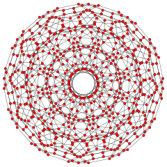
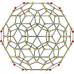
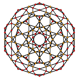
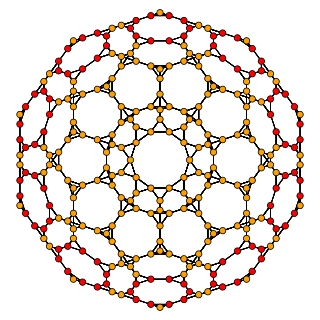
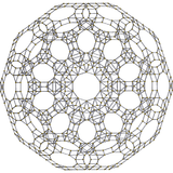
Orthogonal projections
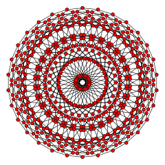
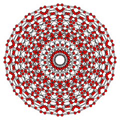
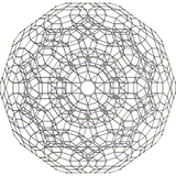
Orthogonal projections of the 120-cell can be done in 2D by defining two orthonormal basis vectors for a specific view direction. The 30-gonal projection was made in 1963 by B. L.Chilton.[7]
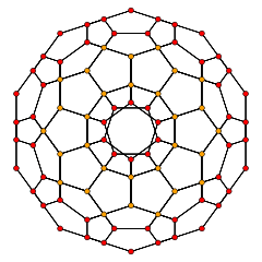
The H3 decagonal projection shows the plane of the van Oss polygon.
| H4 | - | F4 |
|---|---|---|
 [30] |
 [20] |
 [12] |
| H3 | A2 / B3 / D4 | A3 / B2 |
 [10] |
 [6] |
 [4] |
3-dimensional orthogonal projections can also be made with three orthonormal basis vectors, and displayed as a 3d model, and then projecting a certain perspective in 3D for a 2d image.
 3D isometric projection |
Animated 4D rotation |
Perspective projections
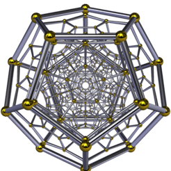
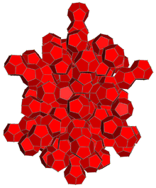
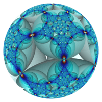
These projections use perspective projection, from a specific view point in four dimensions, and projecting the model as a 3D shadow. Therefore, faces and cells that look larger are merely closer to the 4D viewpoint. Schlegel diagrams use perspective to show four-dimensional figures, choosing a point above a specific cell, thus making the cell as the envelope of the 3D model, and other cells are smaller seen inside it. Stereographic projection use the same approach, but are shown with curved edges, representing the polytope a tiling of a 3-sphere.
A comparison of perspective projections from 3D to 2D is shown in analogy.
| Projection | Dodecahedron | Dodecaplex |
|---|---|---|
| Schlegel diagram | 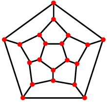 12 pentagon faces in the plane |
120 dodecahedral cells in 3-space |
| Stereographic projection | 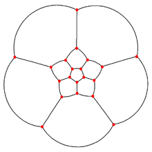 |
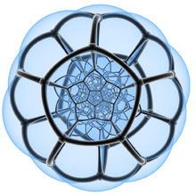 With transparent faces |
| Perspective projection | |
|---|---|
 |
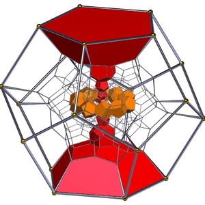
Cell-first perspective projection at 5 times the distance from the center to a vertex, with these enhancements applied:
|
 |
Vertex-first perspective projection at 5 times the distance from center to a vertex, with these enhancements:
|
 |
A 3D projection of a 120-cell performing a simple rotation. |
 |
A 3D projection of a 120-cell performing a simple rotation (from the inside). |
| Animated 4D rotation | |
Related polyhedra and honeycombs
The 120-cell is one of 15 regular and uniform polytopes with the same symmetry [3,3,5]:
| H4 family polytopes | |||||||||||
|---|---|---|---|---|---|---|---|---|---|---|---|
| 120-cell | rectified 120-cell |
truncated 120-cell |
cantellated 120-cell |
runcinated 120-cell |
cantitruncated 120-cell |
runcitruncated 120-cell |
omnitruncated 120-cell | ||||
| {5,3,3} | r{5,3,3} | t{5,3,3} | rr{5,3,3} | t0,3{5,3,3} | tr{5,3,3} | t0,1,3{5,3,3} | t0,1,2,3{5,3,3} | ||||
|
 |
 |
 |
 |
 |
 |
 | ||||
 |
 |
 |
 |
 |
 |
 | |||||
| 600-cell | rectified 600-cell |
truncated 600-cell |
cantellated 600-cell |
bitruncated 600-cell |
cantitruncated 600-cell |
runcitruncated 600-cell |
omnitruncated 600-cell | ||||
| {3,3,5} | r{3,3,5} | t{3,3,5} | rr{3,3,5} | 2t{3,3,5} | tr{3,3,5} | t0,1,3{3,3,5} | t0,1,2,3{3,3,5} | ||||
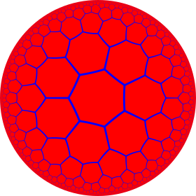
It is similar to three regular 4-polytopes: the 5-cell {3,3,3}, tesseract {4,3,3}, of Euclidean 4-space, and hexagonal tiling honeycomb of hyperbolic space. All of these have a tetrahedral vertex figure.
| {p,3,3} polytopes | |||||||||||
|---|---|---|---|---|---|---|---|---|---|---|---|
| Space | S3 | H3 | |||||||||
| Form | Finite | Paracompact | Noncompact | ||||||||
| Name | {3,3,3} | {4,3,3} | {5,3,3} | {6,3,3} | {7,3,3} | {8,3,3} | ...{∞,3,3} | ||||
| Image |  |
 |
|
 |
 |
 |
 | ||||
| Cells {p,3} |
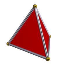 {3,3} |
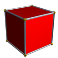 {4,3} |
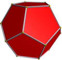 {5,3} |
 {6,3} |
 {7,3} |
 {8,3} |
 {∞,3} | ||||
This honeycomb is a part of a sequence of 4-polytopes and honeycombs with dodecahedral cells:
| {5,3,p} polytopes | |||||||
|---|---|---|---|---|---|---|---|
| Space | S3 | H3 | |||||
| Form | Finite | Compact | Paracompact | Noncompact | |||
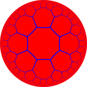
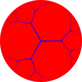
| Name | {5,3,3} | {5,3,4} | {5,3,5} | {5,3,6} | {5,3,7} | {5,3,8} | ... {5,3,∞} |
| Image | |
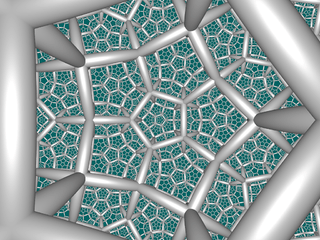 |
 |
 |
 |
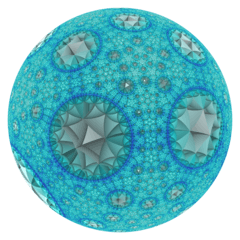 |
 |
| Vertex figure |
{3,3} |
{3,4} |
{3,5} |
{3,6} |
{3,7} |
{3,8} |
{3,∞} |
In popular culture
The video game Deltarune (2018) mentions the hyperdodecahedron on a poster, contrasting with various two-dimensional shapes. During a skit in Battle for Dream Island (2018), a pair of characters plays Rock paper scissors together. When a third character joins in, he doesn’t understand the rules, and makes various illegal moves physically impossible for the human hand, such as the hecatonicosahedroid.
See also
- Uniform 4-polytope family with [5,3,3] symmetry
- 57-cell – an abstract regular 4-polytope constructed from 57 hemi-dodecahedra.
- 600-cell - the dual 4-polytope to the 120-cell
Notes
- N.W. Johnson: Geometries and Transformations, (2018) ISBN 978-1-107-10340-5 Chapter 11: Finite Symmetry Groups, 11.5 Spherical Coxeter groups, p.249
- Matila Ghyka, The Geometry of Art and Life (1977), p.68
- Coxeter, Regular polytopes, p.293
- Coxeter, Regular Polytopes, sec 1.8 Configurations
- Coxeter, Complex Regular Polytopes, p.117
- Weisstein, Eric W. "120-cell". MathWorld.
- "B.+L.+Chilton"+polytopes On the projection of the regular polytope {5,3,3} into a regular triacontagon, B. L. Chilton, Nov 29, 1963.
References
- H. S. M. Coxeter, Regular Polytopes, 3rd. ed., Dover Publications, 1973. ISBN 0-486-61480-8.
- Kaleidoscopes: Selected Writings of H.S.M. Coxeter, edited by F. Arthur Sherk, Peter McMullen, Anthony C. Thompson, Asia Ivic Weiss, Wiley-Interscience Publication, 1995, ISBN 978-0-471-01003-6
- (Paper 22) H.S.M. Coxeter, Regular and Semi-Regular Polytopes I, [Math. Zeit. 46 (1940) 380-407, MR 2,10]
- (Paper 23) H.S.M. Coxeter, Regular and Semi-Regular Polytopes II, [Math. Zeit. 188 (1985) 559-591]
- (Paper 24) H.S.M. Coxeter, Regular and Semi-Regular Polytopes III, [Math. Zeit. 200 (1988) 3-45]
- J.H. Conway and M.J.T. Guy: Four-Dimensional Archimedean Polytopes, Proceedings of the Colloquium on Convexity at Copenhagen, page 38 und 39, 1965
- Davis, Michael W. (1985), "A hyperbolic 4-manifold", Proceedings of the American Mathematical Society, 93 (2): 325–328, doi:10.2307/2044771, ISSN 0002-9939, JSTOR 2044771, MR 0770546
- N.W. Johnson: The Theory of Uniform Polytopes and Honeycombs, Ph.D. Dissertation, University of Toronto, 1966
- Four-dimensional Archimedean Polytopes (German), Marco Möller, 2004 PhD dissertation
External links
- Weisstein, Eric W. "120-Cell". MathWorld.
- Olshevsky, George. "Hecatonicosachoron". Glossary for Hyperspace. Archived from the original on 4 February 2007.
- Klitzing, Richard. "4D uniform polytopes (polychora) o3o3o5x - hi".
- Der 120-Zeller (120-cell) Marco Möller's Regular polytopes in R4 (German)
- 120-cell explorer – A free interactive program that allows you to learn about a number of the 120-cell symmetries. The 120-cell is projected to 3 dimensions and then rendered using OpenGL.
- Construction of the Hyper-Dodecahedron
- YouTube animation of the construction of the 120-cell Gian Marco Todesco.
| H4 family polytopes | |||||||||||
|---|---|---|---|---|---|---|---|---|---|---|---|
| 120-cell | rectified 120-cell |
truncated 120-cell |
cantellated 120-cell |
runcinated 120-cell |
cantitruncated 120-cell |
runcitruncated 120-cell |
omnitruncated 120-cell | ||||
| {5,3,3} | r{5,3,3} | t{5,3,3} | rr{5,3,3} | t0,3{5,3,3} | tr{5,3,3} | t0,1,3{5,3,3} | t0,1,2,3{5,3,3} | ||||
|
|
|
|
|
|
|
| ||||
|
|
|
|
|
|
| |||||
| 600-cell | rectified 600-cell |
truncated 600-cell |
cantellated 600-cell |
bitruncated 600-cell |
cantitruncated 600-cell |
runcitruncated 600-cell |
omnitruncated 600-cell | ||||
| {3,3,5} | r{3,3,5} | t{3,3,5} | rr{3,3,5} | 2t{3,3,5} | tr{3,3,5} | t0,1,3{3,3,5} | t0,1,2,3{3,3,5} | ||||
Fundamental convex regular and uniform polytopes in dimensions 2–10 | ||||||||||||
|---|---|---|---|---|---|---|---|---|---|---|---|---|
| Family | An | Bn | I2(p) / Dn | E6 / E7 / E8 / F4 / G2 | Hn | |||||||
| Regular polygon | Triangle | Square | p-gon | Hexagon | Pentagon | |||||||
| Uniform polyhedron | Tetrahedron | Octahedron • Cube | Demicube | Dodecahedron • Icosahedron | ||||||||
| Uniform 4-polytope | 5-cell | 16-cell • Tesseract | Demitesseract | 24-cell | 120-cell • 600-cell | |||||||
| Uniform 5-polytope | 5-simplex | 5-orthoplex • 5-cube | 5-demicube | |||||||||
| Uniform 6-polytope | 6-simplex | 6-orthoplex • 6-cube | 6-demicube | 122 • 221 | ||||||||
| Uniform 7-polytope | 7-simplex | 7-orthoplex • 7-cube | 7-demicube | 132 • 231 • 321 | ||||||||
| Uniform 8-polytope | 8-simplex | 8-orthoplex • 8-cube | 8-demicube | 142 • 241 • 421 | ||||||||
| Uniform 9-polytope | 9-simplex | 9-orthoplex • 9-cube | 9-demicube | |||||||||
| Uniform 10-polytope | 10-simplex | 10-orthoplex • 10-cube | 10-demicube | |||||||||
| Uniform n-polytope | n-simplex | n-orthoplex • n-cube | n-demicube | 1k2 • 2k1 • k21 | n-pentagonal polytope | |||||||
| Topics: Polytope families • Regular polytope • List of regular polytopes and compounds | ||||||||||||