Function (mathematics)

In mathematics, a function^[1] was originally the idealization of how a varying quantity depends on another quantity. For example, the position of a planet is a function of time. Historically, the concept was elaborated with the infinitesimal calculus at the end of the 17th century, and, until the 19th century, the functions that were considered were differentiable (that is, they had a high degree of regularity). The concept of function was formalized at the end of the 19th century in terms of set theory, and this greatly enlarged the domains of application of the concept.

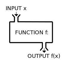
A function is a process or a relation that associates each element $x$ of a set $X$ , the domain of the function, to a single element $y$ of another set $Y$ (possibly the same set), the codomain of the function. If the function is called $f$ , this relation is denoted $y = f (x)$ (read $f$ of $x$ ), the element $x$ is the argument or input of the function, and $y$ is the value of the function, the output, or the image of $x$ by $f$ .^[2] The symbol that is used for representing the input is the variable of the function (one often says that $f$ is a function of the variable $x$ ).

A function is uniquely represented by its graph which is the set of all pairs $(x, f (x))$ . When the domain and the codomain are sets of numbers, each such pair may be considered as the Cartesian coordinates of a point in the plane. In general, these points form a curve, which is also called the graph of the function. This is a useful representation of the function, which is commonly used everywhere, for example in newspapers.

Functions are widely used in science, and in most fields of mathematics. Their role is so important that it has been said that they are "the central objects of investigation" in most fields of mathematics.^[3]

Metaphor describing a function as a "machine" or "black box" that for each input returns a corresponding output.

The red curve is the graph of a function, because any vertical line has exactly one crossing point with the curve.

A function that associates any of the four colored shapes to its color.

Definition

Diagram of a function, with domain X={1, 2, 3} and codomain Y={A, B, C, D}, which is defined by the set of ordered pairs {(1,D), (2,C), (3,C)}. The image/range is the set {C,D}.

This diagram, representing the set of pairs {(1,D), (2,B), (2,C)}, does not define a function. One reason is that 2 is the first element in more than one ordered pair, (2, B) and (2, C), of this set. Two other reasons, also sufficient by themselves, is that neither 3 nor 4 are first elements (input) of any ordered pair therein.

Intuitively, a function is a process that associates to each element of a set $X$ a unique element of a set $Y$ .

Formally, a function $f$ from a set $X$ to a set $Y$ is defined by a set $G$ of ordered pairs $(x, y)$ such that $x \in X$ , $y \in Y$ , and every element of $X$ is the first component of exactly one ordered pair in $G$ .^[4] In other words, for every $x$ in $X$ , there is exactly one element $y$ such that the ordered pair $(x, y)$ belongs to the set of pairs defining the function $f$ . The set $G$ is called the graph of the function. Formally speaking, it may be identified with the function, but this hides the usual interpretation of a function as a process. Therefore, in common usage, the function is generally distinguished from its graph. Functions are also called maps or mappings. However, some authors^[5] reserve the word mapping to the case where the codomain Y belongs explicitly to the definition of the function. In this sense, the graph of the mapping recovers the function as the set of pairs.

In the definition of function, $X$ and $Y$ are respectively called the domain and the codomain of the function $f$ . If $(x, y)$ belongs to the set defining $f$ , then $y$ is the image of $x$ under $f$ , or the value of $f$ applied to the argument $x$ . Especially in the context of numbers, one says also that $y$ is the value of $f$ for the value $x$ of its variable, or, still shorter, $y$ is the value of $f$ of $x$ , denoted as $y = f (x)$ .

The domain and codomain are not always explicitly given when a function is defined, and, without some (possibly difficult) computation, one knows only that the domain is contained in a larger set. Typically, this occurs in mathematical analysis, where "a function from $X$ to $Y$ " often refers to a function that may have a proper subset of $X$ as domain. For example, a "function from the reals to the reals" may refer to a real-valued function of a real variable, and this phrase does not mean that the domain of the function is the whole set of the real numbers, but only that the domain is a set of real numbers that contains a non-empty open interval. For example, if $f$ is a function that has the real numbers as domain and codomain, then a function mapping the value $x$ to the value $g(x)={\tfrac {1}{f(x)}}$ is a function $g$ from the reals to the reals, whose domain is the set of the reals $x$ , such that $f (x) \neq 0$ . In many cases, the exact domains are difficult to determine, but this is rarely a problem for working with such functions.

The range of a function is the set of the images of all elements in the domain. However, range is sometimes used as a synonym of codomain, generally in old textbooks.

Relational approach

Any subset of the Cartesian product of a domain $X$ and a codomain $Y$ is said to define a binary relation $R\subseteq (X\times Y)$ between these two sets. It is immediate that an arbitrary relation may contain pairs that violate the necessary conditions for a function, given above.

A univalent relation is a relation such that

(x,y)\in R\;\land \;(x,z)\in R\quad \Rightarrow \quad y=z.

Univalent relations may be identified to functions whose domain is a subset of $X$ .

A left-total relation is a relation such that

\forall x\in X\;\exists y\in Y:\;(x,y)\in R.

Formal functions may be strictly identified to relations that are both univalent and left total. Violating the left-totality is similar to giving a convenient encompassing set instead of the true domain, as explained above.

Various properties of functions and also the functional composition may be reformulated in the language of relations. For example, a function is injective if the converse relation $R^{\text{T}}\subseteq (Y\times X)$ is univalent, where the converse relation is defined as $R^{\text{T}}=\{(y,x):\;(x,y)\in R\}.$ ^[6]

Notation

There are various standard ways for denoting functions. The most commonly used notation is functional notation, which defines the function using an equation that gives the names of the function and the argument explicitly. This gives rise to a subtle point, often glossed over in elementary treatments of functions: functions are distinct from their values. Thus, a function $f$ should be distinguished from its value $f (x 0)$ at the value $x 0$ in its domain. To some extent, even working mathematicians will conflate the two in informal settings for convenience, and to avoid the use of pedantic language. However, strictly speaking, it is an abuse of notation to write "let $f:\mathbb {R} \to \mathbb {R}$ be the function $f (x) = x 2$ ", since $f (x)$ and $x 2$ should both be understood as the value of f at x, rather than the function itself. Instead, it is correct, though pedantic, to write "let $f:\mathbb {R} \to \mathbb {R}$ be the function defined by the equation $f (x) = x 2,$ valid for all real values of $x$ ".

This distinction in language and notation becomes important in cases where functions themselves serve as inputs for other functions. (A function taking another function as an input is termed a functional.) Other approaches to denoting functions, detailed below, avoid this problem but are less commonly used.

Functional notation

For working with a particular function, it is very often useful to use a symbol for denoting it. This symbol consists generally of a single letter in italic font, most often the lower-case letters $f, g, h$ . Some widely used functions are represented by a symbol consisting of several letters (usually two or three, generally an abbreviation of their name). By convention, the symbol for standard functions is set in roman type, such as " $sin$ " for the sine function, in contrast to functions defined on an ad hoc basis.

The notation (read: " $y$ equals $f$ of $x$ ")

y=f(x)

means that the pair $(x, y)$ belongs to the set of pairs defining the function $f$ . If $X$ is the domain of $f$ , the set of pairs defining the function is thus, using set-builder notation,

\{(x,f(x))\colon x\in X\}.

Often, a definition of the function is given by what f does to the explicit argument x. For example, a function f can be defined by the equation

f(x)=\sin(x^{2}+1)

for all real numbers x. In this example, f can be thought of as the composite of several simpler functions: squaring, adding 1, and taking the sine. However, only the sine function has a common explicit symbol (sin), while the combination of squaring and then adding 1 is described by the polynomial expression $x^{2}+1$ . In order to explicitly reference functions such as squaring or adding 1 without introducing new function names (e.g., by defining function g and h by $g(x)=x^{2}$ and $h(x)=x+1$ ), one of the methods below (arrow notation or dot notation) could be used.

Sometimes the parentheses of the functional notation are omitted, when the symbol denoting the function consists of several characters and no ambiguity may arise, as for

\sin x\quad {\text{instead of}}\quad \sin(x).

Arrow notation

For explicitly expressing domain $X$ and the codomain $Y$ of a function $f$ , the arrow notation is often used (read: "the function $f$ from $X$ to $Y$ " or "the function $f$ mapping elements of $X$ to elements of $Y$ "):

f\colon X\to Y

or

X~{\stackrel {f}{\to }}~Y.

This is often used in relation with the arrow notation for elements (read: " $f$ maps $x$ to $f (x)$ "), often stacked immediately below the arrow notation giving the function symbol, domain, and codomain:

x\mapsto f(x).

For example, if a multiplication is defined on a set $X$ , then the square function $\operatorname {sqr}$ on $X$ is unambiguously defined by (read: "the function $\operatorname {sqr}$ from $X$ to $X$ that maps $x$ to $x \cdot x$ ")

{\begin{aligned}\operatorname {sqr} :X&\to X\\x&\mapsto x\cdot x,\end{aligned}}

the latter line being more commonly written

x\mapsto x^{2}.

Often, the expression giving the function symbol, domain and codomain is omitted. Thus, the arrow notation is useful for avoiding introducing a symbol for a function that is defined, as it is often the case, by a formula expressing the value of the function in terms of its argument. As a common application of the arrow notation, suppose $f:X\times X\to Y;\;(x,t)\mapsto f(x,t)$ is a two-argument function, and we want to refer to a partially applied function $X\to Y$ produced by fixing the second argument to the value $t 0$ without introducing a new function name. The map in question could be denoted $x\mapsto f(x,t_{0})$ using the arrow notation for elements. Note that the expression $x\mapsto f(x,t_{0})$ (read: "the map taking $x$ to $f(x,t_{0})$ ") represents this new function with just one argument, whereas the expression $f(x_{0},t_{0})$ refers to the value of the function $f$ at the point $(x_{0},t_{0})$ .

Index notation

Index notation is often used instead of functional notation. That is, instead of writing $f (x)$ , one writes $f_{x}.$

This is typically the case for functions whose domain is the set of the natural numbers. Such a function is called a sequence, and, in this case the element $f_{n}$ is called the $n$ th element of sequence.

The index notation is also often used for distinguishing some variables called parameters from the "true variables". In fact, parameters are specific variables that are considered as being fixed during the study of a problem. For example, the map $x\mapsto f(x,t)$ (see above) would be denoted $f_{t}$ using index notation, if we define the collection of maps $f_{t}$ by the formula $f_{t}(x)=f(x,t)$ for all $x,t\in X$ .

Dot notation

In the notation $x\mapsto f(x),$ the symbol $x$ does not represent any value, it is simply a placeholder meaning that, if $x$ is replaced by any value on the left of the arrow, it should be replaced by the same value on the right of the arrow. Therefore, $x$ may be replaced by any symbol, often an interpunct " $\cdot$ ". This may be useful for distinguishing the function $f (\cdot)$ from its value $f (x)$ at $x$ .

For example, $a(\cdot )^{2}$ may stand for the function $x\mapsto ax^{2}$ , and $\textstyle \int _{a}^{\,(\cdot )}f(u)\,du$ may stand for a function defined by an integral with variable upper bound: $\textstyle x\mapsto \int _{a}^{x}f(u)\,du$ .

Specialized notations

There are other, specialized notations for functions in sub-disciplines of mathematics. For example, in linear algebra and functional analysis, linear forms and the vectors they act upon are denoted using a dual pair to show the underlying duality. This is similar to the use of bra–ket notation in quantum mechanics. In logic and the theory of computation, the function notation of lambda calculus is used to explicitly express the basic notions of function abstraction and application. In category theory and homological algebra, networks of functions are described in terms of how they and their compositions commute with each other using commutative diagrams that extend and generalize the arrow notation for functions described above.

Specifying a function

According to the definition of a function, a specific function is, in general, defined by associating to every element of its domain at least one element of its codomain. When the domain and the codomain are sets of numbers, this association may take the form of a computation taking as input any element of the domain and producing as output in the codomain. This computation may be described by a formula. (This is the starting point of algebra, which replaces many similar numerical computations by a single formula that describes these computations by a formula involving variables, which represent computation inputs as unspecified numbers). This kind of definition of a function frequently uses previously defined auxiliary functions.

For example, the function $f$ from the reals to the reals, defined by the formula $f(x)={\sqrt {1+x^{2}}},$ employs, as auxiliary functions, the square function (mapping all the reals to the non-negative reals), the square root function (mapping the non-negative reals to the non-negative reals), and the addition of real numbers. The whole set of real numbers may be taken as the domain of $f$ , even if the domain of the square root function is restricted to the non-negative real numbers; the image of $f$ consists of the reals that are not less than one.

The computation that allows defining a function may often be described by an algorithm, and any kind of algorithm may be used. Sometimes, the definition of a function may involve elements or properties that can be defined, but not computed. For example, if one considers the set ${\mathcal {P}}$ of the programs in a given programming language, which take an integer as input. The terminating function is the function that returns 1 if a program of ${\mathcal {P}}$ runs for ever when executed on a given integer input, and returns 0 otherwise. It is a basic theorem of computability theory that it cannot exist an algorithm for computing this function. More generally, the computability theory is the study of the computable functions, that is the functions that can be computed by an algorithm.

Above ways of defining functions define them "pointwise", that is, each value is defined independently of the other values. This is not necessarily the case.

When the domain of a function is the set of nonnegative integers or, more generally, when the domain is well ordered, a function may be defined by induction or recursion, which means (roughly) that the calculation of the value of a function for some given input requires values of the function for lesser inputs. For example, the Fibonacci sequence is a function from the natural numbers into themselves that is defined by two start values and a formula, recurring to the two immediately preceding arguments (see above for the use of indices for the argument of a function):

F_{0}=0,\quad F_{1}=1,\quad {\text{and}}\quad F_{n}=F_{n-1}+F_{n-2}\quad {\text{for }}n>1.

In calculus, the considered functions have extensive regularities. That is, the value of the function at a point is related with the values of the function at neighboring points. This allows defining them by functional equations (for example, the gamma function is the unique meromorphic function such that $\Gamma (1)=1$ , and $\Gamma(z+1)=z\Gamma(z)$ for any complex $z$ that is not a non-positive integer), by differential equations (for example, the natural logarithm is the solution of the differential equation ${\frac {d(\ln x)}{dx}}={\frac {1}{x}}$ such that $ln(1) = 0$ ), integral equations or analytic continuation.

Representing a function

As functions may be complicated objects, it is often useful to draw the graph of a function for getting a global view of its properties. Some functions may also represented histograms

Graph

Given a function $f:X\to Y,$ its graph is, formally, the set

G=\{(x,y):x\in X{\text{ and }}y=f(x)\}.

In the frequent case where $X$ and $Y$ are subsets of the real numbers (or may be identified to such subsets), an element $(x,y)\in G$ may be identified with the point of coordinates $x, y$ in the Cartesian plane. Marking these points provides a drawing, generally a curve, that is also called the graph of the function. For example the graph of the square function

x\mapsto x^2

is a parabola that consists of all points of coordinates $(x,x^{2})$ for $x\in \mathbb {R} .$

It is possible to draw effectively the graph of a function only if the function is sufficiently regular, that is, either if the function is differentiable (or piecewise differentiable) or if its domain may be identified with the integers or a subset of the integers.

If either the domain or the codomain of the function is a subset of $\mathbb {R} ^{n},$ the graph is a subset of a Cartesian space of higher dimension, and various technics have been developed for drawing it, including the use of colors for representing one of the dimensions.

Histogram

Histograms are often used for representing functions whose domain is finite, or is the natural numbers or the integers. In this case, an element $x$ of the domain is represented by an interval of the $x$ -axis, and a point $(x, y)$ of the graph is represented by a rectangle with basis the interval corresponding to $x$ and height $y$ .

In statistic, histogram are often used for representing very irregular functions. For example, for representing the function that associates his weight to each member of some population, one draws the histogram of the function that associates to each weight interval the number of people, whose weights belong to this interval.

There are many variants of this method, see Histogram for details.

General properties

In this section, we describe general properties of functions, that are independent of specific properties of the domain and the codomain.

Canonical functions

Some functions are uniquely defined by their domain and codomain, and are sometimes called canonical:

For every set $X$ , there is a unique function, called the empty function from the empty set to $X$ . This function is not interesting by itself, but useful for simplifying statements, similarly as the empty sum (equal to 0) and the empty product equal to 1.
For every set $X$ and every singleton set ${s}$ , there is a unique function, called the canonical surjection, from $X$ to ${s}$ , which maps to $s$ every element of $X$ . This is a surjection (see below), except if $X$ is the empty set.
Given a function $f\colon X\to Y,$ the canonical surjection of $f$ onto its image $f(X)=\{f(x)\mid x\in X\}$ is the function from $X$ to $f (X)$ that maps $x$ to $f (x)$
For every subset $X$ of a set $Y$ , the canonical injection of $X$ into $Y$ is the injective (see below) function that maps every element of $X$ to itself.
The identity function of $X$ , often denoted by $\operatorname {id} _{X}$ is the canonical injection of $X$ into itself.

Function composition

Given two functions $f:X\to Y$ and $g:Y\to Z$ such that the domain of $g$ is the codomain of $f$ , their composition is the function $g\circ f\colon X\rightarrow Z$ defined by

(g\circ f)(x)=g(f(x)).

That is, the value of $g\circ f$ is obtained by first applying $f$ to $x$ to obtain $y = f (x)$ and then applying $g$ to the result $y$ to obtain $g (y) = g (f (x))$ . In the notation the function that is applied first is always written on the right.

The composition $g\circ f$ is an operation on functions that is defined only if the codomain of the first function is the domain of the second one. Even when $g\circ f$ and $f\circ g$ are both defined, the composition is not commutative. For example, if $f (x) = x 2$ and $g (x) = x + 1$ , one has $g(f(x))=x^{2}+1\neq f(g(x))=(x+1)^{2}.$

The function composition is associative in the sense that, if one of $(h\circ g)\circ f$ and $h\circ (g\circ f)$ is defined, then the other is also defined, and they are equal. Thus, one writes

h\circ g\circ f=(h\circ g)\circ f=h\circ (g\circ f).

The identity functions $\operatorname {id} _{X}$ and $\operatorname {id} _{Y}$ are respectively a right identity and a left identity for functions from $X$ to $Y$ . That is, if $f$ is a function with domain $X$ , and codomain $Y$ , one has $f\circ \operatorname {id} _{X}=\operatorname {id} _{Y}\circ f=f.$

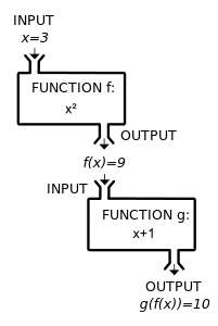A composite function g(f(x)) can be visualized as the combination of two "machines".
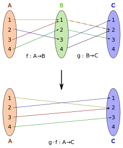A simple example of a function composition
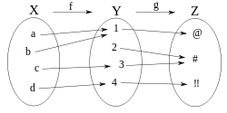Another composition. For example, we have here $(g \circ f)(c) = #$ .

Image and preimage

Let $f\colon X\to Y.$ The image by $f$ of an element $x$ of the domain $X$ is $f (x)$ . If $A$ is any subset of $X$ , then the image of $A$ by $f$ , denoted $f (A)$ is the subset of the codomain $Y$ consisting of all images of elements of $A$ , that is,

f(A)=\{f(x)\mid x\in A\}.

The image of $f$ is the image of the whole domain, that is $f (X)$ . It is also called the range of $f$ , although the term may also refer to the codomain.^[7]

On the other hand, the inverse image, or preimage by $f$ of a subset $B$ of the codomain $Y$ is the subset of the domain $X$ consisting of all elements of $X$ whose images belong to $B$ . It is denoted by $f^{-1}(B).$ That is

f^{-1}(B)=\{x\in X\mid f(x)\in B\}.

For example, the preimage of {4, 9} under the square function is the set {−3,−2,2,3}.

By definition of a function, the image of an element $x$ of the domain is always a single element of the codomain. However, the preimage of a single element $y$ , denoted $f^{-1}(x),$ may be empty or contain any number of elements. For example, if $f$ is the function from the integers to themselves that map every integer to 0, then $f -1 (0) = Z$ .

If $f\colon X\to Y$ is a function, $A$ and $B$ are subsets of $X$ , and $C$ and $D$ are subsets of $Y$ , then one has the following properties:

$A\subseteq B\Longrightarrow f(A)\subseteq f(B)$
$C\subseteq D\Longrightarrow f^{-1}(C)\subseteq f^{-1}(D)$
$A\subseteq f^{-1}(f(A))$
$C\supseteq f(f^{-1}(C))$
$f(f^{-1}(f(A)))=f(A)$
$f^{-1}(f(f^{-1}(C)))=f^{-1}(C)$

The preimage by $f$ of an element $y$ of the codomain is sometimes called, in some contexts, the fiber of $y$ under $f$ .

If a function $f$ has an inverse (see below), this inverse is denoted $f^{-1}.$ In this case $f^{-1}(C)$ may denote either the image by $f^{-1}$ or the preimage by $f$ of $C$ . This is not a problem, as these sets are equal. The notation $f(A)$ and $f^{-1}(C)$ may be ambiguous in the case of sets that contain some subsets as elements, such as $\{x,\{x\}\}.$ In this case, some care may be needed, for example, by using square brackets $f[A],f^{-1}[C]$ for images and preimages of subsets, and ordinary parentheses for images and preimages of elements.

Injective, surjective and bijective functions

Let $f\colon X\to Y$ be a function.

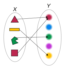
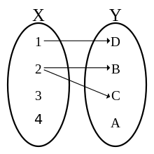
The function $f$ is injective (or one-to-one, or is an injection) if $f (a) \neq f (b)$ for any two different elements $a$ and $b$ of $X$ . Equivalently, $f$ is injective if, for any $y\in Y,$ the preimage $f^{-1}(y)$ contains at most one element. An empty function is always injective. If $X$ is not the empty set, and if, as usual, the axiom of choice is assumed, then $f$ is injective if and only if there exists a function $g\colon y\to X$ such that $g\circ f=\operatorname {id} _{X},$ that is, if $f$ has a left inverse. The axiom of choice is needed, because, if $f$ is injective, one defines $g$ by $g(y)=x$ if $y=f(x),$ and by $g(y)=x_{0}$ , if $y\not \in f(X),$ where $x_{0}$ is an arbitrarily chosen element of $X$ .

The function $f$ is surjective (or onto, or is a surjection) if the range equals the codomain, that is, if $f (X) = Y$ . In other words, the preimage $f^{-1}(y)$ of every $y\in Y$ is nonempty. If, as usual, the axiom of choice is assumed, then $f$ is surjective if and only if there exists a function $g\colon y\to X$ such that $f\circ g=\operatorname {id} _{Y},$ that is, if $f$ has a right inverse. The axiom of choice is needed, because, if $f$ is injective, one defines $g$ by $g(y)=x,$ where $x$ is an arbitrarily chosen element of $f^{-1}(y).$

The function $f$ is bijective (or is bijection or a one-to-one correspondence) if it is both injective and surjective. That is $f$ is bijective if, for any $y\in Y,$ the preimage $f^{-1}(y)$ contains exactly one element. The function $f$ is bijective if and only if it admits an inverse function, that is a function $g\colon y\to X$ such that $g\circ f=\operatorname {id} _{X},$ and $f\circ g=\operatorname {id} _{Y}.$ (Contrarily to the case of injections and surjections, this does not require the axiom of choice.)

Every function $f\colon X\to Y$ may be factorized as the composition $i \circ s$ of a surjection followed by an injection, where $s$ is the canonical surjection of $X$ onto $f (X)$ , and $i$ is the canonical injection of $f (X)$ into $Y$ . This is the canonical factorization of $f$ .

"One-to-one" and "onto" are terms that were more common in the older English language literature; "injective", "surjective", and "bijective" were originally coined as French words in the second quarter of the 20th century by the Bourbaki group and imported into English. As a word of caution, "a one-to-one function" is one that is injective, while a "one-to-one correspondence" refers to a bijective function. Also, the statement " $f$ maps $X$ onto $Y$ " differs from " $f$ maps $X$ into $B$ " in that the former implies that $f$ is surjective), while the latter makes no assertion about the nature of $f$ the mapping. In a complicated reasoning, the one letter difference can easily be missed. Due to the confusing nature of this older terminology, these terms have declined in popularity relative to the Bourbakian terms, which have also the advantage to be more symmetrical.

Restriction and extension

If $f\colon X\to Y$ is a function, and $S$ is a subset of $X$ , then the restriction of $f$ to $S$ , denoted $f | S$ , is the function from $S$ to $Y$ that is defined by

f_{|S}(x)=f(x)\quad {\text{for all }}x\in S.

This often used for define partial inverse functions: if there is a subset $S$ of a function $f$ such that $f | S$ is injective, then the canonical surjection of $f | S$ on its image $f | S (S) = f (S)$ is a bijection, which has an inverse function from $f (S)$ to $S$ . This is in this way that inverse trigonometric functions are defined. The cosine function, for example, is injective, when restricted to the interval $(-0, π)$ ; the image of this restriction is the interval $(-1, 1)$ ; this defines thus an inverse function from $(-1, 1)$ to $(-0, π)$ , which is called arccosine and denoted $arccos$ .

Function restriction may also be used for "gluing" functions together: let $\textstyle X=\bigcup _{i\in I}U_{i}$ be the decomposition of $X$ as a union of subsets. Suppose that a function $f_{i}\colon U_{i}\to Y$ is defined on each $U_{i},$ such that, for each pair of indices, the restrictions of $f_{i}$ and $f_{j}$ to $U_{i}\cap U_{j}$ are equal. Then, this defines a unique function $f\colon X\to Y$ such that $f_{|U_{i}}=f_{i}$ for every $i$ . This is generally in this way that functions on manifolds are defined.

An extension of a function $f$ is a function $g$ such that $f$ is a restriction of $g$ . A typical use of this concept is the process of analytic continuation, that allows extending functions whose domain is a small part of the complex plane to functions whose domain is almost the whole complex plane.

Here is another classical example of a function extension that is encountered when studying homographies of the real line. An homography is a function $h(x)={\frac {ax+b}{cx+d}}$ such that $ad - bc \neq 0$ . Its domain is the set of all real numbers different from $-d/c,$ and its image is the set of all real numbers different from $a/c.$ If one extends the real line to the projectively extended real line by adding $\infty$ to the real numbers, one may extend $h$ for being a bijection of the extended real line to itself, by setting $h(\infty )=a/c$ and $h(-d/c)=\infty .$

Multivariate function

A binary operation is a typical example of a bivariate, function which assigns to each pair

(x,y)

the result

x\circ y

.

A multivariate function, or function of several variables is a function that depends on several arguments. Such functions are commonly encountered. For example, the position of a car on a road is a function of the time and its speed.

More formally, a function of $n$ variables is a function whose domain is a set of $n$ -tuples. For example, multiplication of integers is a function of two variables, or bivariate function, whose domain is the set of all pairs (2-tuples) of integers, and whose codomain is the set of integers. The same is true for every binary operation. More generally, every mathematical operation is defined as a multivariate function.

The Cartesian product $X_{1}\times \cdots \times X_{n}$ of $n$ sets $X_1, \ldots, X_n$ is the set of all $n$ -tuples $(x_1, \ldots, x_n)$ such that $x_{i}\in X_{i}$ for every $i$ with $1\leq i\leq n$ . Therefore, a function of $n$ variables is a function

f:U\to Y,

where the domain $U$ has the form

U\subseteq X_{1}\times \cdots \times X_{n}.

When using function notation, one usually omits the parentheses surrounding tuples, writing $f(x_1,x_2)$ instead of $f((x_{1},x_{2})).$

In the case where all the $X_{i}$ are equal to the set $\mathbb {R}$ of real numbers, one has a function of several real variables. If the $X_{i}$ are equal to the set $\mathbb {C}$ of complex numbers, one has a function of several complex variables.

It is common to also consider functions whose codomain is a product of sets. For example, Euclidean division maps every pair $(a, b)$ of integers with $b \neq 0$ to a pair of integers called the quotient and the remainder:

{\begin{aligned}{\text{Euclidean division}}\colon \quad \mathbb {Z} \times (\mathbb {Z} \setminus \{0\})&\to \mathbb {Z} \times \mathbb {Z} \\(a,b)&\mapsto (\operatorname {quotient} (a,b),\operatorname {remainder} (a,b)).\end{aligned}}

The codomain may also be a vector space. In this case, one talks of a vector-valued function. If the domain is contained in a Euclidean space, or more generally a manifold, a vector-valued function is often called a vector field.

In calculus

The idea of function, starting in the 17th century, was fundamental to the new infinitesimal calculus (see History of the function concept). At that time, only real-valued functions of a real variable were considered, and all functions were assumed to be smooth. But the definition was soon extended to functions of several variables and to function of a complex variable. In the second half of 19th century, the mathematically rigorous definition of a function was introduced, and functions with arbitrary domains and codomains were defined.

Functions are now used throughout all areas of mathematics. In introductory calculus, when the word function is used without qualification, it means a real-valued function of a single real variable. The more general definition of a function is usually introduced to second or third year college students with STEM majors, and in their senior year they are introduced to calculus in a larger, more rigorous setting in courses such as real analysis and complex analysis.

Real function

Graph of a linear function

Graph of a polynomial function, here a quadratic function.

Graph of two trigonometric functions: sine and cosine.

A real function is a real-valued function of a real variable, that is, a function whose codomain is the field of real numbers and whose domain is a set of real numbers that contains an interval. In this section, these functions are simply called functions.

The functions that are most commonly considered in mathematics and its applications have some regularity, that is they are continuous, differentiable, and even analytic. This regularity insures that these functions can be visualized by their graphs. In this section, all functions are differentiable in some interval.

Functions enjoy pointwise operations, that is, if $f$ and $g$ are functions, their sum, difference and product are functions defined by

{\begin{aligned}(f+g)(x)&=f(x)+g(x)\\(f-g)(x)&=f(x)-g(x)\\(f\cdot g)(x)&=f(x)\cdot g(x)\\\end{aligned}}.

The domains of the resulting functions are the intersection of the domains of $f$ and $g$ . The quotient of two functions is defined similarly by

{\frac {f}{g}}(x)={\frac {f(x)}{g(x)}},

but the domain of the resulting function is obtained by removing the zeros of $g$ from the intersection of the domains of $f$ and $g$ .

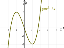
The polynomial functions are defined by polynomials, and their domain is the whole set of real numbers. They include constant functions, linear functions and quadratic functions. Rational functions are quotients of two polynomial functions, and their domain is the real numbers with a finite number of them removed to avoid division by zero. The simplest rational function is the function $x\mapsto {\frac {1}{x}},$ whose graph is an hyperbola, and whose domain is the whole real line except for 0.

The derivative of a real differentiable function is a real function. An antiderivative of a continuous real function is a real function that is differentiable in any open interval in which the original function is continuous. For example, the function $x\mapsto {\frac {1}{x}}$ is continuous, and even differentiable, on the positive real numbers. Thus one antiderivative, which takes the value zero for $x = 1$ , is a differentiable function called the natural logarithm.

A real function $f$ is monotonic in an interval if the sign of ${\frac {f(x)-f(y)}{x-y}}$ does not depend of the choice of $x$ and $y$ in the interval. If the function is differentiable in the interval, it is monotonic if the sign of the derivative is constant in the interval. If a real function $f$ is monotonic in an interval $I$ , it has an inverse function, which is a real function with domain $f (I)$ and image $I$ . This is how inverse trigonometric functions are defined in terms of trigonometric functions, where the trigonometric functions are monotonic. Another example: the natural logarithm is monotonic on the positive real numbers, and its image is the whole real line; therefore it has an inverse function that is a bijection between the real numbers and the positive real numbers. This inverse is the exponential function.

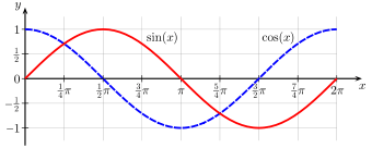
Many other real functions are defined either by the implicit function theorem (the inverse function is a particular instance) or as solutions of differential equations. For example the sine and the cosine functions are the solutions of the linear differential equation

y''+y=0

such that

\sin 0=0,\quad \cos 0=1,\quad {\frac {\partial \sin x}{\partial x}}(0)=1,\quad {\frac {\partial \cos x}{\partial x}}(0)=0.

Complex function

When working with complex numbers different types of functions are used^[8]:

Complex-valued functions, functions that return complex values

f:X\to {\mathbb {C}}

for

X

an arbitrary set, or perhaps a subset of the real numbers.

Or a function for which both domain and range are subsets of the complex numbers.

f:\mathbb {C} \to \mathbb {C}

.

Complex variable functions that return, say real numbers or other values

f:\mathbb {C} \to X

.

The study of complex functions is a vast subject in mathematics with many applications, and that can claim^[9] to be an ancestor to many other areas of mathematics, like homotopy theory, and manifolds.

Function of several real or complex variables

Vector-valued function

Function space

In mathematical analysis, and more specifically in functional analysis, a function space is a set of scalar-valued or vector-valued functions, which share a specific property and form a topological vector space. For example, the real smooth functions with a compact support (that is, they are zero outside some compact set) form a function space that is at the basis of the theory of distributions.

Function spaces play a fundamental role in advanced mathematical analysis, by allowing the use of their algebraic and topological properties for studying properties of functions. For example, all theorems of existence and uniqueness of solutions of ordinary or partial differential equations result of the study of function spaces.

Generalizations

Natural extension

It is rather frequent that a function with domain $X$ may be naturally extended to a function whose domain is a set $Z$ that is built from $X$ .

For example, for any set $X$ , its power set $P (X)$ is the set of all subsets of $X$ . Any function $f:X\to Y,$ may be extended to a function on power sets by

{\begin{aligned}&{\mathcal {P}}(X)\to {\mathcal {P}}(Y)\\&S\mapsto f(S)\end{aligned}}

where $f (S)$ is the image by $f$ of the subset $S$ of $X$ .

According to the definition, a function $f$ maps each element from its domain $X$ to some element of its codomain $Y$ . It is often convenient to extend this meaning to apply to arbitrary subsets of the domain, which are, as immediately can be checked, mapped to subsets of the codomain, thus considering a function ${\tilde {f}},$ mapping its domain, the powerset P( $X$ ) of $f$ 's domain $X$ , to its codomain, a subset of the powerset P( $Y$ ) of $f$ 's codomain $Y$ .

{\begin{aligned}{\mathcal {P}}(X)\to {\mathcal {P}}(Y)\\S\mapsto f(S).\end{aligned}}

Under slight abuse of notation this function on subsets is often denoted also by $f$ .

Another example is the following. If the function $f:R\to S$ is a ring homomorphism, it may be extended to a function on polynomial rings

{\begin{aligned}R[x]&\to S[x]\\\sum _{i=0}^{n}a_{i}x^{i}&\mapsto \sum _{i=0}^{n}f(a_{i})x^{i},\end{aligned}}

which is also a ring homomorphism.

Multi-valued functions

Together, the two square roots of all nonnegative real numbers form a single smooth curve.

Several methods for specifying functions of real or complex variables start from a local definition of the funcion at a point or on a neighbourhood of a point, and then extend by continuity the function to a much larger domain. Frequently, for a starting point $x_0,$ there are several possible starting values for the function.

For example, in defining the square root as the inverse function of the square function, for any positive real number $x_0,$ there are two choices for the value of the square root, one of which is positive and denoted ${\sqrt {x_{0}}},$ and another which is negative and denoted $-{\sqrt {x_{0}}}.$ These choices define two continuous functions, both having the nonnegative real numbers as a domain, and having either the nonnegative or the nonpositive real numbers as images. When looking at the graphs of these functions, one can see that, together, they form a single smooth curve. It is therefore often useful to consider these two square root functions as a single function that has two values for positive $x$ , one value for 0 and no value for negative $x$ .

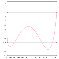
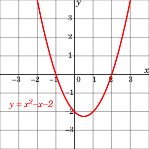
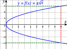
In the preceding example, one choice, the positive square root, is more natural than the other. This is not the case in general. For example, let consider the implicit function that maps $y$ to a root $x$ of $x^{3}-3x-y=0$ (see the figure on the right). For $y = 0$ one may choose either $0,{\sqrt {3}},{\text{ or }}-{\sqrt {3}}$ for $x.$ By the implicit function theorem, each choice defines a function; for the first one, the (maximal) domain is the interval $[-2, 2]$ and the image is $[-1, 1]$ ; for the second one, the domain is $[-2, \infty)$ and the image is $[1, \infty)$ ; for the last one, the domain is $(-\infty, 2]$ and the image is $(-\infty, -1]$ . As the three graphs together form a smooth curve, and there is no reason for preferring one choice, these three functions are often considered as a single multi-valued function of $y$ that has three values for $-2 < y < 2$ , and only one value for $y \leq -2$ and $y \geq -2$ .

Usefulness of the concept of multi-valued functions is clearer when considering complex functions, typically analytic functions. The domain to which a complex function is analytic may be extended by analytic continuation consists generally of almost the whole complex plane. However, it is frequent that, when extending the domain through two different paths, one gets different values. For example, when extending the domaine of the square root function, along a path of complex numbers with positive imaginary parts, one gets $i$ for the square root of –1, while, when extending through complex numbers with negative imaginary parts, one gets $- i$ . There are generally two ways for solving the problem. One may define a function that is not continuous along some curve, called branch cut. Such a function is called the principal value of the function. The other way is to consider that one has a multi-valued function, which is analytic everywhere except for isolated singularities, but whose value may "jump" if one follows a closed loop around a singularity. This jump is called the monodromy.

In foundations of mathematics and set theory

The definition of a function that is given in this article requires the concept of set, since the domain and the codomain of a function must be a set. This is not a problem in usual mathematics, as it is generally not difficult to consider only functions whose domain and codomain are sets, which are well defined, even if the domain is not explicitly defined. However, it is sometimes useful to consider more general functions.

For example the singleton set may be considered as a function $x\mapsto \{x\}.$ Its domain would include all sets, and therefore would not be a set. In usual mathematics, one avoids this kind of problem by specifying a domain, which means that one has many singleton functions. However, when establishing foundations of mathematics, one may have to use functions whose domain, codomain or both are not specified, and some authors, often logicians, give precise definition for these weakly specified functions.^[10]

These generalized functions may be critical in the development of a formalization of foundations of mathematics. For example, the Von Neumann–Bernays–Gödel set theory, is an extension of the set theory in which the collection of all sets is a class. This theory includes the replacement axiom, which may be interpreted as "if $X$ is a set, and $F$ is a function, then $F [X]$ is a set".

In computer science

↑ The words map, mapping, transformation, correspondence, and operator are often used synonymously. Halmos 1970, p. 30.
↑ MacLane, Saunders; Birkhoff, Garrett (1967). Algebra (First ed.). New York: Macmillan. pp. 1–13.
↑ Spivak 2008, p. 39.
↑ Hamilton, A. G. Numbers, sets, and axioms: the apparatus of mathematics. Cambridge University Press. p. 83. ISBN 0-521-24509-5.
↑ T. M. Apostol (1981). Mathematical Analysis. Addison-Wesley. p. 35.
↑ Gunther Schmidt( 2011) Relational Mathematics, Encyclopedia of Mathematics and its Applications, vol. 132, sect 5.1 Functions, pages 49 to 60, Cambridge University Press ISBN 978-0-521-76268-7 CUP blurb for Relational Mathematics
↑ Quantities and Units - Part 2: Mathematical signs and symbols to be used in the natural sciences and technology, page 15. ISO 80000-2 (ISO/IEC 2009-12-01)
↑ L. Ahlfors (1966). Complex Analysis (second ed.). McGraw-Hill. p. 21.
↑ J. B. Conway (1978). Functions of one complex variable (second ed.). Springer-Verlag. p. vii.
↑ Gödel 1940, p. 16; Jech 2003, p. 11; Cunningham 2016, p. 57

References

Bartle, Robert (1967). The Elements of Real Analysis. John Wiley & Sons.
Bloch, Ethan D. (2011). Proofs and Fundamentals: A First Course in Abstract Mathematics. Springer. ISBN 978-1-4419-7126-5.
Cunningham, Daniel W. (2016). Set theory: A First Course. Cambridge University Press. ISBN 978-1107120327.
Gödel, Kurt (1940). The Consistency of the Continuum Hypothesis. Princeton University Press. ISBN 978-0691079271.
Halmos, Paul R. (1970). Naive Set Theory. Springer-Verlag. ISBN 0-387-90092-6.
Jech, Thomas (2003). Set theory (Third Millennium ed.). Springer-Verlag. ISBN 3-540-44085-2.
Spivak, Michael (2008). Calculus (4th ed.). Publish or Perish. ISBN 978-0-914098-91-1.

External links

Hazewinkel, Michiel, ed. (2001) [1994], "Function", Encyclopedia of Mathematics, Springer Science+Business Media B.V. / Kluwer Academic Publishers, ISBN 978-1-55608-010-4
Weisstein, Eric W. "Function". MathWorld.
The Wolfram Functions Site gives formulae and visualizations of many mathematical functions.
NIST Digital Library of Mathematical Functions

This article is issued from Wikipedia. The text is licensed under Creative Commons - Attribution - Sharealike. Additional terms may apply for the media files.

[1] The words map, mapping, transformation, correspondence, and operator are often used synonymously. Halmos 1970, p. 30.

[MacLane-2] MacLane, Saunders; Birkhoff, Garrett (1967). Algebra (First ed.). New York: Macmillan. pp. 1–13.

[FOOTNOTESpivak200839-3] Spivak 2008, p. 39.

[4] Hamilton, A. G. Numbers, sets, and axioms: the apparatus of mathematics. Cambridge University Press. p. 83. ISBN 0-521-24509-5.

[5] T. M. Apostol (1981). Mathematical Analysis. Addison-Wesley. p. 35.

[RM-6] Gunther Schmidt( 2011) Relational Mathematics, Encyclopedia of Mathematics and its Applications, vol. 132, sect 5.1 Functions, pages 49 to 60, Cambridge University Press ISBN 978-0-521-76268-7 CUP blurb for Relational Mathematics

[standard-7] Quantities and Units - Part 2: Mathematical signs and symbols to be used in the natural sciences and technology, page 15. ISO 80000-2 (ISO/IEC 2009-12-01)

[8] L. Ahlfors (1966). Complex Analysis (second ed.). McGraw-Hill. p. 21.

[9] J. B. Conway (1978). Functions of one complex variable (second ed.). Springer-Verlag. p. vii.

[10] Gödel 1940, p. 16; Jech 2003, p. 11; Cunningham 2016, p. 57

Mathematical logic
General	Formal language Formation rule Formal proof Formal semantics Well-formed formula Set Element Class Classical logic Axiom Rule of inference Relation Theorem Logical consequence Type theory Symbol Syntax Theory
Systems	Formal system Deductive system Axiomatic system Hilbert style systems Natural deduction Sequent calculus
Traditional logic	Proposition Inference Argument Validity Cogency Syllogism Square of opposition Venn diagram
Propositional calculus and Boolean logic	Boolean functions Propositional calculus Propositional formula Logical connectives Truth tables Many-valued logic
Predicate logic	First-order Quantifiers Predicate Second-order Monadic predicate calculus
Naive set theory	Set Empty set Element Enumeration Extensionality Finite set Infinite set Subset Power set Countable set Uncountable set Recursive set Domain Codomain Image Map Function Relation Ordered pair
Set theory	Foundations of mathematics Zermelo–Fraenkel set theory Axiom of choice General set theory Kripke–Platek set theory Von Neumann–Bernays–Gödel set theory Morse–Kelley set theory Tarski–Grothendieck set theory
Model theory	Model Interpretation Non-standard model Finite model theory Truth value Validity
Proof theory	Formal proof Deductive system Formal system Theorem Logical consequence Rule of inference Syntax
Computability theory	Recursion Recursive set Recursively enumerable set Decision problem Church–Turing thesis Computable function Primitive recursive function

Function (mathematics)

Definition

Relational approach

Notation

Functional notation

Arrow notation

Index notation

Dot notation

Specialized notations

Specifying a function

Representing a function

Graph

Histogram

General properties

Canonical functions

Function composition

Image and preimage

Injective, surjective and bijective functions

Restriction and extension

Multivariate function

In calculus

Real function

Complex function

Function of several real or complex variables

Vector-valued function

Function space

Generalizations

Natural extension

Multi-valued functions

In foundations of mathematics and set theory

In computer science

See also

Subpages

Generalizations

Related topics

Notes

References

Further reading

External links