Square root

The mathematical expression "The (principal) square root of x"

For example,

\sqrt 25 = 5

, since

25 = 5 \cdot 5

, or

52

(5 squared).

In mathematics, a square root of a number a is a number y such that y² = a; in other words, a number y whose square (the result of multiplying the number by itself, or y⋅y) is a.^[1] For example, 4 and −4 are square roots of 16 because 4² = (−4)² = 16. Every nonnegative real number a has a unique nonnegative square root, called the principal square root, which is denoted by √a, where √ is called the radical sign or radix. For example, the principal square root of 9 is 3, which is denoted by √9 = 3, because 3² = 3 • 3 = 9 and 3 is nonnegative. The term (or number) whose square root is being considered is known as the radicand. The radicand is the number or expression underneath the radical sign, in this example 9.

Every positive number a has two square roots: √a, which is positive, and −√a, which is negative. Together, these two roots are denoted as ± √a (see ± shorthand). Although the principal square root of a positive number is only one of its two square roots, the designation "the square root" is often used to refer to the principal square root. For positive a, the principal square root can also be written in exponent notation, as a^1/2.^[2]

Square roots of negative numbers can be discussed within the framework of complex numbers. More generally, square roots can be considered in any context in which a notion of "squaring" of some mathematical objects is defined (including algebras of matrices, endomorphism rings, etc.)

History

The Yale Babylonian Collection YBC 7289 clay tablet was created between 1800 BC and 1600 BC, showing √2 and √2/2 = 1/√2 as 1;24,51,10 and 0;42,25,35 base 60 numbers on a square crossed by two diagonals.^[3] (1;24,51,10) base 60 corresponds to 1.41421296 which is a correct value to 5 decimal points (1.41421356...).

The Rhind Mathematical Papyrus is a copy from 1650 BC of an earlier Berlin Papyrus and other texts – possibly the Kahun Papyrus – that shows how the Egyptians extracted square roots by an inverse proportion method.^[4]

In Ancient India, the knowledge of theoretical and applied aspects of square and square root was at least as old as the Sulba Sutras, dated around 800–500 BC (possibly much earlier). A method for finding very good approximations to the square roots of 2 and 3 are given in the Baudhayana Sulba Sutra.^[5] Aryabhata in the Aryabhatiya (section 2.4), has given a method for finding the square root of numbers having many digits.

It was known to the ancient Greeks that square roots of positive whole numbers that are not perfect squares are always irrational numbers: numbers not expressible as a ratio of two integers (that is to say they cannot be written exactly as m/n, where m and n are integers). This is the theorem Euclid X, 9 almost certainly due to Theaetetus dating back to circa 380 BC.^[6] The particular case √2 is assumed to date back earlier to the Pythagoreans and is traditionally attributed to Hippasus. It is exactly the length of the diagonal of a square with side length 1.

In the Chinese mathematical work Writings on Reckoning, written between 202 BC and 186 BC during the early Han Dynasty, the square root is approximated by using an "excess and deficiency" method, which says to "...combine the excess and deficiency as the divisor; (taking) the deficiency numerator multiplied by the excess denominator and the excess numerator times the deficiency denominator, combine them as the dividend."^[7]

A symbol for square roots, written as an elaborate R, was invented by Regiomontanus (1436–1476). An R was also used for Radix to indicate square roots in Gerolamo Cardano's Ars Magna.^[8]

According to historian of mathematics D.E. Smith, Aryabhata's method for finding the square root was first introduced in Europe by Cataneo in 1546.

According to Jeffrey A. Oaks, Arabs used the letter jīm/ĝīm (ج), the first letter of the word “جذر” (variously transliterated as jaḏr, jiḏr, ǧaḏr or ǧiḏr, “root”), placed in its initial form (ﺟ) over a number to indicate its square root. The letter jīm resembles the present square root shape. Its usage goes as far as the end of the twelfth century in the works of the Moroccan mathematician Ibn al-Yasamin.^[9]

The symbol '√' for the square root was first used in print in 1525 in Christoph Rudolff's Coss.^[10]

Properties and uses

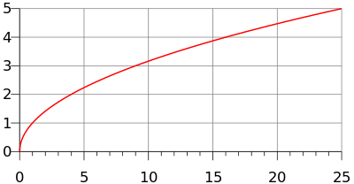
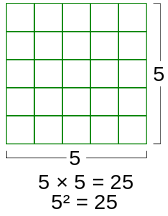
The graph of the function f(x) = √x, made up of half a parabola with a vertical directrix

The principal square root function f(x) = √x (usually just referred to as the "square root function") is a function that maps the set of nonnegative real numbers onto itself. In geometrical terms, the square root function maps the area of a square to its side length.

The square root of x is rational if and only if x is a rational number that can be represented as a ratio of two perfect squares. (See square root of 2 for proofs that this is an irrational number, and quadratic irrational for a proof for all non-square natural numbers.) The square root function maps rational numbers into algebraic numbers (a superset of the rational numbers).

For all real numbers x

\sqrt{x^2} = \left|x\right| = \begin{cases} x, & \mbox{if }x \ge 0 \\ -x, & \mbox{if }x < 0. \end{cases}

(see absolute value)

For all nonnegative real numbers x and y,

\sqrt{xy} = \sqrt x \sqrt y

and

\sqrt x = x^{1/2}.

The square root function is continuous for all nonnegative x and differentiable for all positive x. If f denotes the square root function, its derivative is given by:

f'(x) = \frac{1}{2\sqrt x}.

The Taylor series of √1 + x about x = 0 converges for |x| ≤ 1 and is given by

{\sqrt {1+x}}=\sum _{n=0}^{\infty }{\frac {(-1)^{n}(2n)!}{(1-2n)(n!)^{2}(4^{n})}}x^{n}=1+\textstyle {\frac {1}{2}}x-{\frac {1}{8}}x^{2}+{\frac {1}{16}}x^{3}-{\frac {5}{128}}x^{4}+\dots ,

The square root of a nonnegative number is used in the definition of Euclidean norm (and distance), as well as in generalizations such as Hilbert spaces. It defines an important concept of standard deviation used in probability theory and statistics. It has a major use in the formula for roots of a quadratic equation; quadratic fields and rings of quadratic integers, which are based on square roots, are important in algebra and have uses in geometry. Square roots frequently appear in mathematical formulas elsewhere, as well as in many physical laws.

Computation

Most pocket calculators have a square root key. Computer spreadsheets and other software are also frequently used to calculate square roots. Pocket calculators typically implement efficient routines, such as the Newton's method (frequently with an initial guess of 1), to compute the square root of a positive real number.^[11]^[12] When computing square roots with logarithm tables or slide rules, one can exploit the identities

{\sqrt {a}}=e^{(\ln a)/2}=10^{(\log _{10}a)/2},

where $ln$ and $log$ ₁₀ are the natural and base-10 logarithms.

By trial-and-error,^[13] one can square an estimate for √a and raise or lower the estimate until it agrees to sufficient accuracy. For this technique it's prudent to use the identity

(x+c)^{2}=x^{2}+2xc+c^{2},

as it allows one to adjust the estimate x by some amount c and measure the square of the adjustment in terms of the original estimate and its square. Furthermore, (x + c)² ≈ x² + 2xc when c is close to 0, because the tangent line to the graph of x² + 2xc + c² at c=0, as a function of c alone, is y = 2xc + x². Thus, small adjustments to x can be planned out by setting 2xc to a, or c=a/(2x).

The most common iterative method of square root calculation by hand is known as the "Babylonian method" or "Heron's method" after the first-century Greek philosopher Heron of Alexandria, who first described it.^[14] The method uses the same iterative scheme as the Newton–Raphson method yields when applied to the function y = f(x) = x² − a, using the fact that its slope at any point is dy/dx = f'(x) = 2x, but predates it by many centuries.^[15] The algorithm is to repeat a simple calculation that results in a number closer to the actual square root each time it is repeated with its result as the new input. The motivation is that if x is an overestimate to the square root of a nonnegative real number a then a/x will be an underestimate and so the average of these two numbers is a better approximation than either of them. However, the inequality of arithmetic and geometric means shows this average is always an overestimate of the square root (as noted below), and so it can serve as a new overestimate with which to repeat the process, which converges as a consequence of the successive overestimates and underestimates being closer to each other after each iteration. To find x:

Start with an arbitrary positive start value x. The closer to the square root of a, the fewer the iterations that will be needed to achieve the desired precision.
Replace x by the average (x + a/x) / 2 between x and a/x.
Repeat from step 2, using this average as the new value of x.

That is, if an arbitrary guess for √a is x₀, and x_{n + 1} = (x_n + a/x_n) / 2, then each x_n is an approximation of √a which is better for large n than for small n. If a is positive, the convergence is quadratic, which means that in approaching the limit, the number of correct digits roughly doubles in each next iteration. If a = 0, the convergence is only linear.

Using the identity

\sqrt{a} = 2^{-n}\sqrt{4^n a},

the computation of the square root of a positive number can be reduced to that of a number in the range $[1,4)$ . This simplifies finding a start value for the iterative method that is close to the square root, for which a polynomial or piecewise-linear approximation can be used.

The time complexity for computing a square root with n digits of precision is equivalent to that of multiplying two n-digit numbers.

Another useful method for calculating the square root is the shifting nth root algorithm, applied for n = 2.

The name of the square root function varies from programming language to programming language, with sqrt^[16] (often pronounced "squirt" ^[17]) being common, used in C, C++, and derived languages like JavaScript, PHP, and Python.

Square roots of negative and complex numbers

First leaf of the complex square root

Second leaf of the complex square root

Using the Riemann surface of the square root, it is shown how the two leaves fit together

The square of any positive or negative number is positive, and the square of 0 is 0. Therefore, no negative number can have a real square root. However, it is possible to work with a more inclusive set of numbers, called the complex numbers, that does contain solutions to the square root of a negative number. This is done by introducing a new number, denoted by i (sometimes j, especially in the context of electricity where "i" traditionally represents electric current) and called the imaginary unit, which is defined such that i² = −1. Using this notation, we can think of i as the square root of −1, but notice that we also have (−i)² = i² = −1 and so −i is also a square root of −1. By convention, the principal square root of −1 is i, or more generally, if x is any nonnegative number, then the principal square root of −x is

\sqrt{-x} = i \sqrt x.

The right side (as well as its negative) is indeed a square root of −x, since

(i\sqrt x)^2 = i^2(\sqrt x)^2 = (-1)x = -x.

For every non-zero complex number z there exist precisely two numbers w such that w² = z: the principal square root of z (defined below), and its negative.

Square root of an imaginary number

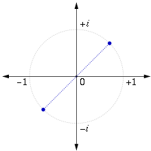
The square roots of i in the complex plane

The square root of $i$ is given by

\sqrt{i} = \frac{1}{2}\sqrt{2} + i\frac{1}{2}\sqrt{2} = \frac{\sqrt{2}}{2}(1+i).

This result can be obtained algebraically by finding real numbers a and b such that

i=(a+bi)^{2}

or equivalently

i=a^{2}+2abi-b^{2}.

This gives the two simultaneous equations

\begin{cases} 2ab = 1\! \\ a^2 - b^2 = 0\! \end{cases}

with solutions

a=b=\pm {\frac {\sqrt {2}}{2}}.

The choice of the principal root then gives

a=b={\frac {\sqrt {2}}{2}}.

The result can also be obtained by using de Moivre's formula and setting

i=\cos \left({\frac {\pi }{2}}\right)+i\sin \left({\frac {\pi }{2}}\right),

which yields

{\begin{aligned}{\sqrt {i}}&=\left(\cos \left({\frac {\pi }{2}}\right)+i\sin \left({\frac {\pi }{2}}\right)\right)^{\frac {1}{2}}\\&=\cos \left({\frac {\pi }{4}}\right)+i\sin \left({\frac {\pi }{4}}\right)\\&={\frac {\sqrt {2}}{2}}+i{\frac {\sqrt {2}}{2}}\\&={\frac {\sqrt {2}}{2}}(1+i).\\\end{aligned}}

Principal square root of a complex number

Visualisation of the square to sixth roots of a complex number z, in polar form re^iφ where φ = arg z and r = |z | – if z is real, φ = 0 or

π

. Principal roots are in black.

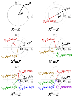
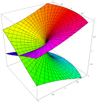
To find a definition for the square root that allows us to consistently choose a single value, called the principal value, we start by observing that any complex number x + iy can be viewed as a point in the plane, (x, y), expressed using Cartesian coordinates. The same point may be reinterpreted using polar coordinates as the pair $(r,\varphi$ ), where r ≥ 0 is the distance of the point from the origin, and $\varphi$ is the angle that the line from the origin to the point makes with the positive real (x) axis. In complex analysis, the location of this point is conventionally written $re^{i\varphi }.$ If

z=re^{{i\varphi }}{\text{ with }}-\pi <\varphi \leq \pi ,

then we define the principal square root of z as follows:

\sqrt{z} = \sqrt{r} \, e^{i \varphi / 2}.

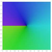
The principal square root function is thus defined using the nonpositive real axis as a branch cut. The principal square root function is holomorphic everywhere except on the set of non-positive real numbers (on strictly negative reals it isn't even continuous). The above Taylor series for √1 + x remains valid for complex numbers x with |x| < 1.

The above can also be expressed in terms of trigonometric functions:

\sqrt{r \left(\cos \varphi + i \, \sin \varphi \right)} = \sqrt{r} \left [ \cos \frac{\varphi}{2} + i \sin \frac{\varphi}{2} \right ] .

Algebraic formula

When the number is expressed using Cartesian coordinates the following formula can be used for the principal square root:^[18]^[19]

{\sqrt {z}}={\sqrt {\frac {|z|+\operatorname {Re} (z)}{2}}}\pm i\ {\sqrt {\frac {|z|-\operatorname {Re} (z)}{2}}},

where the sign of the imaginary part of the root is taken to be the same as the sign of the imaginary part of the original number, or positive when zero. The real part of the principal value is always nonnegative.

Notes

In the following, the complex z and w may be expressed as:

$z=|z|e^{i\theta _{z}}$
$w=|w|e^{i\theta _{w}}$

where $-\pi <\theta _{z}\leq \pi$ and $-\pi <\theta _{w}\leq \pi$ .

Because of the discontinuous nature of the square root function in the complex plane, the following laws are not true in general.

${\sqrt {zw}}={\sqrt {z}}{\sqrt {w}}$ (counterexample for the principal square root: $z = -1$ and $w = -1$ ) This equality is valid only when $-\pi <\theta _{z}+\theta _{w}\leq \pi$
${\frac {\sqrt {w}}{\sqrt {z}}}={\sqrt {\frac {w}{z}}}$ (counterexample for the principal square root: $w = 1$ and $z = -1$ )This equality is valid only when $-\pi <\theta _{w}-\theta _{z}\leq \pi$
${\sqrt {z^{*}}}=\left({\sqrt {z}}\right)^{*}$ (counterexample for the principal square root: $z = -1$ )This equality is valid only when $\theta _{z}\neq \pi$

A similar problem appears with other complex functions with branch cuts, e.g., the complex logarithm and the relations $log z + log w = log(zw)$ or $log (z *) = log (z) *$ which are not true in general.

Wrongly assuming one of these laws underlies several faulty "proofs", for instance the following one showing that $-1 = 1$ :

{\begin{aligned}-1&=i\cdot i\\&={\sqrt {-1}}\cdot {\sqrt {-1}}\\&={\sqrt {\left(-1\right)\cdot \left(-1\right)}}\\&={\sqrt {1}}\\&=1\end{aligned}}

The third equality cannot be justified (see invalid proof). It can be made to hold by changing the meaning of √ so that this no longer represents the principal square root (see above) but selects a branch for the square root that contains (√−1)·(√−1). The left-hand side becomes either

\sqrt{-1} \cdot \sqrt{-1}=i \cdot i=-1

if the branch includes +i or

\sqrt{-1} \cdot \sqrt{-1}=(-i) \cdot (-i)=-1

if the branch includes −i, while the right-hand side becomes

{\sqrt {\left(-1\right)\cdot \left(-1\right)}}={\sqrt {1}}=-1,

where the last equality, $\sqrt 1 = -1$ , is a consequence of the choice of branch in the redefinition of √.

Square roots of matrices and operators

If A is a positive-definite matrix or operator, then there exists precisely one positive definite matrix or operator B with B² = A; we then define A^1/2 = B. In general matrices may have multiple square roots or even an infinitude of them. For example, the 2 × 2 identity matrix has an infinity of square roots,^[20] though only one of them is positive definite.

In integral domains, including fields

Each element of an integral domain has no more than 2 square roots. The difference of two squares identity $u 2 - v 2 = (u - v)(u + v)$ is proved using the commutativity of multiplication. If $u$ and $v$ are square roots of the same element, then $u 2 - v 2 = 0$ . Because there are no zero divisors this implies $u = v$ or $u + v = 0$ , where the latter means that two roots are additive inverses of each other. In other words if an element a square root $u$ of an element $a$ exists, then the only square roots of $a$ are $u$ and $- u$ . The only square root of 0 in an integral domain is 0 itself.

In a field of characteristic 2, an element either has one square root or does not have any at all, because each element is its own additive inverse, so that $- u = u$ . If the field is finite of characteristic 2 then every element has a unique square root. In a field of any other characteristic, any non-zero element either has two square roots, as explained above, or does not have any.

Given an odd prime number $p$ , let $q = p e$ for some positive integer $e$ . A non-zero element of the field $F q$ with $q$ elements is a quadratic residue if it has a square root in $F q$ . Otherwise, it is a quadratic non-residue. There are $(q - 1)/2$ quadratic residues and $(q - 1)/2$ quadratic non-residues; zero is not counted in either class. The quadratic residues form a group under multiplication. The properties of quadratic residues are widely used in number theory.

In rings in general

In a ring we call an element b a square root of a iff b² = a. To see that the square root need not be unique up to sign in a general ring, consider the ring $\mathbb {Z} /8\mathbb {Z}$ from modular arithmetic. Here, the element 1 has four distinct square roots, namely ±1 and ±3. On the other hand, the element 2 has no square root. See also the article quadratic residue for details.

Another example is provided by the quaternions $\mathbb {H}$ in which the element −1 has an infinitude of square roots including ±i, ±j, and ±k.

In fact, the set of square roots of −1 is exactly

\{ai + bj + ck \mid a^2 + b^2 + c^2 = 1\} .

Hence this set is exactly the same size and shape as the unit sphere in 3-space.

The square root of 0 is by definition either 0 or a zero divisor, and where zero divisors do not exist (such as in quaternions and, generally, in division algebras), it is uniquely 0. It is not necessarily true in general rings, where $Z / n 2 Z$ for any natural $n$ provides an easy counterexample.

Principal square roots of the positive integers

As decimal expansions

The square roots of the perfect squares (1, 4, 9, 16, etc.) are integers. In all other cases, the square roots of positive integers are irrational numbers, and therefore their decimal representations are non-repeating decimals.

√0	= 0
√1	= 1
√2	≈ 1.414213562373095048801688724209698078569671875376948073176679737990732478462	(article) 1 million digits, 2 million, 5 million, 10 million
√3	≈ 1.732050807568877293527446341505872366942805253810380628055806979451933016909	(article) 1 million digits, 2 million
√4	= 2
√5	≈ 2.236067977499789696409173668731276235440618359611525724270897245410520925638	(article) 1 million digits
√6	≈ 2.449489742783178098197284074705891391965947480656670128432692567250960377457	1 million digits
√7	≈ 2.645751311064590590501615753639260425710259183082450180368334459201068823230	1 million digits
√8	≈ 2.828427124746190097603377448419396157139343750753896146353359475981464956924	1 million digits
√9	= 3
√10	≈ 3.162277660168379331998893544432718533719555139325216826857504852792594438639	1 million digits
√11	≈ 3.316624790355399849114932736670686683927088545589353597058682146116484642609	10 million digits (verified)
√12	≈ 3.464101615137754587054892683011744733885610507620761256111613958903866033818	500,000 digits
√13	≈ 3.605551275463989293119221267470495946251296573845246212710453056227166948293	200,000 digits
√14	≈ 3.741657386773941385583748732316549301756019807778726946303745467320035156307
√15	≈ 3.872983346207416885179265399782399610832921705291590826587573766113483091937
√16	= 4
√17	≈ 4.123105625617660549821409855974077025147199225373620434398633573094954346338	100,000 digits
√18	≈ 4.242640687119285146405066172629094235709015626130844219530039213972197435386
√19	≈ 4.358898943540673552236981983859615659137003925232444936890344138159557328203	100,000 digits
√20	≈ 4.472135954999579392818347337462552470881236719223051448541794490821041851276
√21	≈ 4.582575694955840006588047193728008488984456576767971902607242123906868425547	100,000 digits

If the radicand is not square-free, then one can factorize, for example

$\sqrt{8} \ = \ \sqrt{4}\sqrt{2} \ = \ 2\sqrt{2}$
$\sqrt{12} \ = \ \sqrt{4}\sqrt{3} \ = \ 2\sqrt{3}$
$\sqrt{18} \ = \ \sqrt{9}\sqrt{2} \ = \ 3\sqrt{2}$
$\sqrt{20} \ = \ \sqrt{4}\sqrt{5} \ = \ 2\sqrt{5}$ .

As expansions in other numeral systems

The square roots of the perfect squares (1, 4, 9, 16, etc.) are integers. In all other cases, the square roots of positive integers are irrational numbers, and therefore their representations in any standard positional notation system are non-repeating.

The square roots of small integers are used in both the SHA-1 and SHA-2 hash function designs to provide nothing up my sleeve numbers.

As periodic continued fractions

One of the most intriguing results from the study of irrational numbers as continued fractions was obtained by Joseph Louis Lagrange c. 1780. Lagrange found that the representation of the square root of any non-square positive integer as a continued fraction is periodic. That is, a certain pattern of partial denominators repeats indefinitely in the continued fraction. In a sense these square roots are the very simplest irrational numbers, because they can be represented with a simple repeating pattern of integers.

√2	= [1; 2, 2, ...]
√3	= [1; 1, 2, 1, 2, ...]
√4	= [2]
√5	= [2; 4, 4, ...]
√6	= [2; 2, 4, 2, 4, ...]
√7	= [2; 1, 1, 1, 4, 1, 1, 1, 4, ...]
√8	= [2; 1, 4, 1, 4, ...]
√9	= [3]
√10	= [3; 6, 6, ...]
√11	= [3; 3, 6, 3, 6, ...]
√12	= [3; 2, 6, 2, 6, ...]
√13	= [3; 1, 1, 1, 1, 6, 1, 1, 1, 1, 6, ...]
√14	= [3; 1, 2, 1, 6, 1, 2, 1, 6, ...]
√15	= [3; 1, 6, 1, 6, ...]
√16	= [4]
√17	= [4; 8, 8, ...]
√18	= [4; 4, 8, 4, 8, ...]
√19	= [4; 2, 1, 3, 1, 2, 8, 2, 1, 3, 1, 2, 8, ...]
√20	= [4; 2, 8, 2, 8, ...]

The square bracket notation used above is a sort of mathematical shorthand to conserve space. Written in more traditional notation the simple continued fraction for the square root of 11, [3; 3, 6, 3, 6, ...], looks like this:

\sqrt{11} = 3 + \cfrac{1}{3 + \cfrac{1}{6 + \cfrac{1}{3 + \cfrac{1}{6 + \cfrac{1}{3 + \ddots}}}}}

where the two-digit pattern {3, 6} repeats over and over again in the partial denominators. Since 11 = 3² + 2, the above is also identical to the following generalized continued fractions:

\sqrt{11} = 3 + \cfrac{2}{6 + \cfrac{2}{6 + \cfrac{2}{6 + \cfrac{2}{6 + \cfrac{2}{6 + \ddots}}}}} = 3 + \cfrac{6\cdot 1}{20-1 - \cfrac{1}{20 - \cfrac{1}{20 - \cfrac{1}{20 - \ddots}}}}.

Geometric construction of the square root

The spiral of Theodorus up to the triangle with a hypotenuse of

\sqrt 4

(

1 = \sqrt 1

)

The square root of a positive number is usually defined as the side length of a square with the area equal to the given number. But the square shape is not necessary for it: if one of two similar planar Euclidean objects has the area a times greater than another, then the ratio of their linear sizes is √a.

A square root can be constructed with a compass and straightedge. In his Elements, Euclid (fl. 300 BC) gave the construction of the geometric mean of two quantities in two different places: Proposition II.14 and Proposition VI.13. Since the geometric mean of a and b is $\sqrt {ab}$ , one can construct ${\sqrt {a}}$ simply by taking b = 1.

The construction is also given by Descartes in his La Géométrie, see figure 2 on page 2. However, Descartes made no claim to originality and his audience would have been quite familiar with Euclid.

Euclid's second proof in Book VI depends on the theory of similar triangles. Let AHB be a line segment of length a + b with AH = a and HB = b. Construct the circle with AB as diameter and let C be one of the two intersections of the perpendicular chord at H with the circle and denote the length CH as h. Then, using Thales' theorem and, as in the proof of Pythagoras' theorem by similar triangles, triangle AHC is similar to triangle CHB (as indeed both are to triangle ACB, though we don't need that, but it is the essence of the proof of Pythagoras' theorem) so that AH:CH is as HC:HB, i.e. $\ a/h = h/b,$ from which we conclude by cross-multiplication that $\ h^2 = ab,$ and finally that $h = \sqrt {ab}$ . When marking the midpoint O of the line segment AB and drawing the radius OC of length $(a + b)/2$ , then clearly OC > CH, i.e. $(a + b)/2 \ge \sqrt {ab}$ (with equality if and only if a = b), which is the arithmetic–geometric mean inequality for two variables and, as noted above, is the basis of the Ancient Greek understanding of "Heron's method".

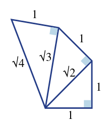
Another method of geometric construction uses right triangles and induction: √1 can, of course, be constructed, and once √x has been constructed, the right triangle with 1 and √x for its legs has a hypotenuse of √x + 1. The Spiral of Theodorus is constructed using successive square roots in this manner.

Notes

↑ Gel'fand, p. 120 Archived 2016-09-02 at the Wayback Machine.
↑ Zill, Dennis G.; Shanahan, Patrick (2008). A First Course in Complex Analysis With Applications (2nd ed.). Jones & Bartlett Learning. p. 78. ISBN 0-7637-5772-1. Archived from the original on 2016-09-01. Extract of page 78 Archived 2016-09-01 at the Wayback Machine.
↑ "Analysis of YBC 7289". ubc.ca. Retrieved 19 January 2015.
↑ Anglin, W.S. (1994). Mathematics: A Concise History and Philosophy. New York: Springer-Verlag.
↑ Joseph, ch.8.
↑ Heath, Sir Thomas L. (1908). The Thirteen Books of The Elements, Vol. 3. Cambridge University Press. p. 3.
↑ Dauben (2007), p. 210.
↑ "The Development of Algebra - 2". maths.org. Archived from the original on 24 November 2014. Retrieved 19 January 2015.
↑
- Oaks, Jeffrey A. (2012). Algebraic Symbolism in Medieval Arabic Algebra (PDF) (Thesis). Philosophica. p. 36. Archived (PDF) from the original on 2016-12-03.
↑ Manguel, Alberto (2006). "Done on paper: the dual nature of numbers and the page". The Life of Numbers. ISBN 84-86882-14-1.
↑ Parkhurst, David F. (2006). Introduction to Applied Mathematics for Environmental Science. Springer. p. 241. ISBN 9780387342283.
↑ Solow, Anita E. (1993). Learning by Discovery: A Lab Manual for Calculus. Cambridge University Press. p. 48. ISBN 9780883850831.
↑ Aitken, Mike; Broadhurst, Bill; Hladky, Stephen (2009). Mathematics for Biological Scientists. Garland Science. p. 41. ISBN 978-1-136-84393-8. Archived from the original on 2017-03-01. Extract of page 41 Archived 2017-03-01 at the Wayback Machine.
↑ Heath, Sir Thomas L. (1921). A History of Greek Mathematics, Vol. 2. Oxford: Clarendon Press. pp. 323–324.
↑ Muller, Jean-Mic (2006). Elementary functions: algorithms and implementation. Springer. pp. 92–93. ISBN 0-8176-4372-9. , Chapter 5, p 92 Archived 2016-09-01 at the Wayback Machine.
↑ "Function sqrt". CPlusPlus.com. The C++ Resources Network. 2016. Archived from the original on November 22, 2012. Retrieved June 24, 2016.
↑ Overland, Brian (2013). C++ for the Impatient. Addison-Wesley. p. 338. ISBN 9780133257120. OCLC 850705706. Archived from the original on September 1, 2016. Retrieved June 24, 2016.
↑ Abramowitz, Milton; Stegun, Irene A. (1964). Handbook of mathematical functions with formulas, graphs, and mathematical tables. Courier Dover Publications. p. 17. ISBN 0-486-61272-4. Archived from the original on 2016-04-23. , Section 3.7.27, p. 17 Archived 2009-09-10 at the Wayback Machine.
↑ Cooke, Roger (2008). Classical algebra: its nature, origins, and uses. John Wiley and Sons. p. 59. ISBN 0-470-25952-3. Archived from the original on 2016-04-23.
↑ Mitchell, Douglas W., "Using Pythagorean triples to generate square roots of I₂", Mathematical Gazette 87, November 2003, 499–500.

References

Dauben, Joseph W. (2007). "Chinese Mathematics I". In Katz, Victor J. The Mathematics of Egypt, Mesopotamia, China, India, and Islam. Princeton: Princeton University Press. ISBN 0-691-11485-4.
Gel'fand, Izrael M.; Shen, Alexander (1993). Algebra (3rd ed.). Birkhäuser. p. 120. ISBN 0-8176-3677-3.
Joseph, George (2000). The Crest of the Peacock. Princeton: Princeton University Press. ISBN 0-691-00659-8.
Smith, David (1958). History of Mathematics. 2. New York: Dover Publications. ISBN 978-0-486-20430-7.
Selin, Helaine (2008), Encyclopaedia of the History of Science, Technology, and Medicine in Non-Western Cultures, Springer, ISBN 978-1-4020-4559-2 .

External links

Algorithms, implementations, and more – Paul Hsieh's square roots webpage
How to manually find a square root
AMS Featured Column, Galileo's Arithmetic by Tony Philips – includes a section on how Galileo found square roots

This article is issued from Wikipedia. The text is licensed under Creative Commons - Attribution - Sharealike. Additional terms may apply for the media files.

[1] Gel'fand, p. 120 Archived 2016-09-02 at the Wayback Machine.

[2] Zill, Dennis G.; Shanahan, Patrick (2008). A First Course in Complex Analysis With Applications (2nd ed.). Jones & Bartlett Learning. p. 78. ISBN 0-7637-5772-1. Archived from the original on 2016-09-01. Extract of page 78 Archived 2016-09-01 at the Wayback Machine.

[3] "Analysis of YBC 7289". ubc.ca. Retrieved 19 January 2015.

[4] Anglin, W.S. (1994). Mathematics: A Concise History and Philosophy. New York: Springer-Verlag.

[5] Joseph, ch.8.

[6] Heath, Sir Thomas L. (1908). The Thirteen Books of The Elements, Vol. 3. Cambridge University Press. p. 3.

[7] Dauben (2007), p. 210.

[8] "The Development of Algebra - 2". maths.org. Archived from the original on 24 November 2014. Retrieved 19 January 2015.

[9] 
Oaks, Jeffrey A. (2012). Algebraic Symbolism in Medieval Arabic Algebra (PDF) (Thesis). Philosophica. p. 36. Archived (PDF) from the original on 2016-12-03.

[mwBAU] Oaks, Jeffrey A. (2012). Algebraic Symbolism in Medieval Arabic Algebra (PDF) (Thesis). Philosophica. p. 36. Archived (PDF) from the original on 2016-12-03.

[10] Manguel, Alberto (2006). "Done on paper: the dual nature of numbers and the page". The Life of Numbers. ISBN 84-86882-14-1.

[11] Parkhurst, David F. (2006). Introduction to Applied Mathematics for Environmental Science. Springer. p. 241. ISBN 9780387342283.

[12] Solow, Anita E. (1993). Learning by Discovery: A Lab Manual for Calculus. Cambridge University Press. p. 48. ISBN 9780883850831.

[13] Aitken, Mike; Broadhurst, Bill; Hladky, Stephen (2009). Mathematics for Biological Scientists. Garland Science. p. 41. ISBN 978-1-136-84393-8. Archived from the original on 2017-03-01. Extract of page 41 Archived 2017-03-01 at the Wayback Machine.

[14] Heath, Sir Thomas L. (1921). A History of Greek Mathematics, Vol. 2. Oxford: Clarendon Press. pp. 323–324.

[15] Muller, Jean-Mic (2006). Elementary functions: algorithms and implementation. Springer. pp. 92–93. ISBN 0-8176-4372-9. , Chapter 5, p 92 Archived 2016-09-01 at the Wayback Machine.

[16] "Function sqrt". CPlusPlus.com. The C++ Resources Network. 2016. Archived from the original on November 22, 2012. Retrieved June 24, 2016.

[17] Overland, Brian (2013). C++ for the Impatient. Addison-Wesley. p. 338. ISBN 9780133257120. OCLC 850705706. Archived from the original on September 1, 2016. Retrieved June 24, 2016.

[18] Abramowitz, Milton; Stegun, Irene A. (1964). Handbook of mathematical functions with formulas, graphs, and mathematical tables. Courier Dover Publications. p. 17. ISBN 0-486-61272-4. Archived from the original on 2016-04-23. , Section 3.7.27, p. 17 Archived 2009-09-10 at the Wayback Machine.

[19] Cooke, Roger (2008). Classical algebra: its nature, origins, and uses. John Wiley and Sons. p. 59. ISBN 0-470-25952-3. Archived from the original on 2016-04-23.

[20] Mitchell, Douglas W., "Using Pythagorean triples to generate square roots of I₂", Mathematical Gazette 87, November 2003, 499–500.