Lambert ''W'' function

The graph of

W (x)

for

W > -4

and

x < 6

. The upper branch with

W \geq -1

is the function

W 0

(principal branch), the lower branch with

W \leq -1

is the function

W -1

.

In mathematics, the Lambert $W$ function, also called the omega function or product logarithm, is a set of functions, namely the branches of the inverse relation of the function $f (z) = ze z$ , where $e z$ is the exponential function, and $z$ is any complex number. In other words

z=f^{-1}\left(ze^{z}\right)=W\left(ze^{z}\right).

By substituting $z 0 = ze z$ into the equation above, we get the defining equation for the $W$ function (and for the $W$ relation in general):

z_{0}=W(z_{0})e^{W(z_{0})}

for any complex number $z 0$ .

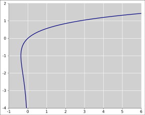
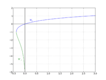
Since the function $f$ is not injective, the relation $W$ is multivalued (except at 0). If we restrict attention to real-valued $W$ , the complex variable $z$ is then replaced by the real variable $x$ , and the relation is defined only for $x \geq - 1 / e$ and is double-valued on $(- 1 / e,0)$ . The additional constraint $W \geq -1$ defines a single-valued function $W 0 (x)$ . We have $W 0 (0) = 0$ and $W 0 (- 1 / e) = -1$ . Meanwhile, the lower branch has $W \leq -1$ and is denoted $W -1 (x)$ . It decreases from $W -1 (- 1 / e) = -1$ to $W -1 (0 -) = -\infty$ .

It can be extended to the function $z = xa x$ using the identity

x={\frac {W(z\ln {a})}{\ln {a}}}.

The Lambert $W$ relation cannot be expressed in terms of elementary functions.^[1] It is useful in combinatorics, for instance, in the enumeration of trees. It can be used to solve various equations involving exponentials (e.g. the maxima of the Planck, Bose–Einstein, and Fermi–Dirac distributions) and also occurs in the solution of delay differential equations, such as $y'(t) = a y (t - 1)$ . In biochemistry, and in particular enzyme kinetics, a closed-form solution for the time-course kinetics analysis of Michaelis–Menten kinetics is described in terms of the Lambert $W$ function.

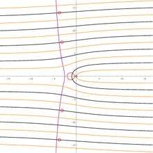
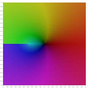Main branch of the Lambert

W

function in the complex plane. Note the branch cut along the negative real axis, ending at

- 1 / e

. In this picture, the hue of a point

z

is determined by the argument of

W (z)

, and the brightness by the absolute value of

W (z)

.

The modulus of the principal branch of the Lambert

W

function, colored according to

arg W (z)

Terminology

The two main branches

W 0

and

W -1

.

The Lambert $W$ function is named after Johann Heinrich Lambert. The main branch $W 0$ is denoted $Wp$ in the Digital Library of Mathematical Functions, and the branch $W -1$ is denoted $Wm$ there.

The notation convention chosen here (with $W 0$ and $W -1$ ) follows the canonical reference on the Lambert $W$ function by Corless, Gonnet, Hare, Jeffrey and Knuth.^[2]

History

Lambert first considered the related Lambert's Transcendental Equation in 1758,^[3] which led to an article by Leonhard Euler in 1783^[4] that discussed the special case of $we w$ .

The function Lambert considered was

x=x^{m}+q.

Euler transformed this equation into the form

x^{a}-x^{b}=(a-b)cx^{a+b}.

Both authors derived a series solution for their equations.

Once Euler had solved this equation he considered the case $a = b$ . Taking limits he derived the equation

\ln x=cx^{a}.

He then put $a = 1$ and obtained a convergent series solution.

After taking derivatives with respect to $x$ and some manipulation, the standard form of the Lambert function is obtained.

In 1993, when it was reported that the Lambert $W$ function provides an exact solution to the quantum-mechanical double-well Dirac delta function model for equal charges—a fundamental problem in physics—Corless and developers of the Maple computer algebra system made a library search and found that this function was ubiquitous in nature.^[2]^[5]

Another example where this function is found is in Michaelis–Menten kinetics.

Calculus

Derivative

By implicit differentiation, one can show that all branches of $W$ satisfy the differential equation

z(1+W){\frac {\mathrm {d} W}{\mathrm {d} z}}=W\quad {\text{for }}z\neq -{\frac {1}{e}}

( $W$ is not differentiable for $z = - 1 / e$ .) As a consequence, we get the following formula for the derivative of W:

{\frac {\mathrm {d} W}{\mathrm {d} z}}={\frac {W(z)}{z(1+W(z))}}\quad {\text{for }}z\not \in \left\{0,-{\frac {1}{e}}\right\}.

Using the identity $e W (z) = z / W (z)$ , we get the following equivalent formula:

{\frac {\mathrm {d} W}{\mathrm {d} z}}={\frac {1}{z+e^{W(z)}}}\quad {\text{for }}z\neq -{\frac {1}{e}}.

Antiderivative

The function $W (x)$ , and many expressions involving $W (x)$ , can be integrated using the substitution $w = W (x)$ , i.e. $x = we w$ :

{\begin{aligned}\int W(x)\,\mathrm {d} x&=xW(x)-x+e^{W(x)}+C\\&=x\left(W(x)-1+{\frac {1}{W(x)}}\right)+C\\\end{aligned}}

(the last equation is more common in the literature but does not hold at $x = 0$ ), one consequence of which (using the fact that $W (e) = 1$ ) is the identity

\int _{0}^{e}W(x)\,\mathrm {d} x=e-1.

Asymptotic expansions

The Taylor series of $W 0$ around 0 can be found using the Lagrange inversion theorem and is given by

W_{0}(x)=\sum _{n=1}^{\infty }{\frac {(-n)^{n-1}}{n!}}x^{n}=x-x^{2}+{\tfrac {3}{2}}x^{3}-{\tfrac {8}{3}}x^{4}+{\tfrac {125}{24}}x^{5}-\cdots

The radius of convergence is $1 / e$ , as may be seen by the ratio test. The function defined by this series can be extended to a holomorphic function defined on all complex numbers with a branch cut along the interval $(-\infty, - 1 / e]$ ; this holomorphic function defines the principal branch of the Lambert $W$ function.

For large values of $x$ , $W 0$ is asymptotic to

{\begin{aligned}W_{0}(x)&=L_{1}-L_{2}+{\frac {L_{2}}{L_{1}}}+{\frac {L_{2}\left(-2+L_{2}\right)}{2L_{1}^{2}}}+{\frac {L_{2}\left(6-9L_{2}+2L_{2}^{2}\right)}{6L_{1}^{3}}}+{\frac {L_{2}\left(-12+36L_{2}-22L_{2}^{2}+3L_{2}^{3}\right)}{12L_{1}^{4}}}+\cdots \\[5pt]&=L_{1}-L_{2}+\sum _{l=0}^{\infty }\sum _{m=1}^{\infty }{\frac {(-1)^{l}\left[{\begin{smallmatrix}l+m\\l+1\end{smallmatrix}}\right]}{m!}}L_{1}^{-l-m}L_{2}^{m},\end{aligned}}

where $L 1 = ln x$ , $L 2 = ln ln x$ , and $[l + m l + 1]$ is a non-negative Stirling number of the first kind.^[6] Keeping only the first two terms of the expansion,

W_{0}(x)=\ln x-\ln \ln x+o(1).

The other real branch, $W -1$ , defined in the interval $[- 1 / e, 0)$ , has an approximation of the same form as $x$ approaches zero, with in this case $L 1 = ln(- x)$ and $L 2 = ln(-ln(- x))$ .

It is shown^[7] that the following bound holds for $x \geq e$ :

\ln x-\ln \ln x+{\frac {\ln \ln x}{2\ln x}}\leq W_{0}(x)\leq \ln x-\ln \ln x+{\frac {e}{e-1}}{\frac {\ln \ln x}{\ln x}}.

In 2016 it was proven^[8] that the branch $W -1$ can be bounded as follows:

-1-{\sqrt {2u}}-u<W_{-1}\left(-e^{-u-1}\right)<-1-{\sqrt {2u}}-{\tfrac {2}{3}}u\quad {\text{for }}u>0.

Integer and complex powers

Integer powers of $W 0$ also admit simple Taylor (or Laurent) series expansions at zero:

W_{0}(x)^{2}=\sum _{n=2}^{\infty }{\frac {-2\left(-n\right)^{n-3}}{(n-2)!}}x^{n}=x^{2}-2x^{3}+4x^{4}-{\tfrac {25}{3}}x^{5}+18x^{6}-\cdots

More generally, for $r \in ℤ$ , the Lagrange inversion formula gives

W_{0}(x)^{r}=\sum _{n=r}^{\infty }{\frac {-r\left(-n\right)^{n-r-1}}{(n-r)!}}x^{n},

which is, in general, a Laurent series of order $r$ . Equivalently, the latter can be written in the form of a Taylor expansion of powers of $W 0 (x) / x$ :

\left({\frac {W_{0}(x)}{x}}\right)^{r}=e^{-rW_{0}(x)}=\sum _{n=0}^{\infty }{\frac {r\left(n+r\right)^{n-1}}{n!}}\left(-x\right)^{n},

which holds for any $r \in ℂ$ and $| x | < 1 / e$ .

Identities

A few identities follow from definition:

{\begin{aligned}W(xe^{x})&=x&{\text{for }}x&\geq 0,\\W_{0}(xe^{x})&=x&{\text{for }}x&\geq -1,\\W_{-1}(xe^{x})&=x&{\text{for }}x&\leq -1.\end{aligned}}

Note that, since $f (x) = xe x$ is not injective, it does not always hold that $W (f (x)) = x$ , much like with the inverse trigonometric functions. For fixed $x < 0$ and $x \neq -1$ the equation $xe x = ye y$ has two solutions in $y$ , one of which is of course $y = x$ . Then, for $i = 0$ and $x < -1$ , as well as for $i = -1$ and $x \in (-1, 0)$ , $y = W i (xe x)$ is the other solution.

Some other identities:^[9]

{\begin{aligned}&W(x)\cdot e^{W(x)}=x,\quad {\text{therefore:}}\\[5pt]&e^{W(x)}={\frac {x}{W(x)}},\qquad e^{-W(x)}={\frac {W(x)}{x}},\qquad e^{nW(x)}=\left({\frac {x}{W(x)}}\right)^{n}.\end{aligned}}

\ln W(x)=\ln x-W(x)\quad {\text{for }}x>0.

^[10]

W\left(a\ln a\right)=\ln a\quad {\text{for }}a\in \mathbb {R} .

{\begin{aligned}&W(x)=\ln {\frac {x}{W(x)}}&&{\text{for }}x\geq {\frac {-1}{e}},\\[5pt]&W\left({\frac {nx^{n}}{W\left(x\right)^{n-1}}}\right)=nW(x)&&{\text{for }}n,x>0\end{aligned}}

(which can be extended to other

n

and

x

if the right branch is chosen).

W(x)+W(y)=W\left(xy\left({\frac {1}{W(x)}}+{\frac {1}{W(y)}}\right)\right)\quad {\text{for }}x,y>0.

From inverting $f (ln x)$ :

{\begin{aligned}W(x\ln x)&=\ln x\\&=W(x)+\ln W(x)\quad {\text{for }}x>0.\end{aligned}}

Substituting $-ln x$ in the definition:

{\begin{aligned}W_{0}\left(-{\frac {\ln x}{x}}\right)&=-\ln x&{\text{for }}0&<x\leq e,\\[5pt]W_{-1}\left(-{\frac {\ln x}{x}}\right)&=-\ln x&{\text{for }}x&>e.\end{aligned}}

With Euler's iterated exponential $h (x)$ :

{\begin{aligned}h(x)&=e^{-W(-\ln x)}\\&={\frac {W(-\ln x)}{-\ln x}}\quad {\text{for }}x\neq 1.\end{aligned}}

Special values

For any nonzero algebraic number $x$ , $W (x)$ is a transcendental number. Indeed, if $W (x)$ is zero, then $x$ must be zero as well, and if $W (x)$ is nonzero and algebraic, then by the Lindemann–Weierstrass theorem, $e W (x)$ must be transcendental, implying that $x = W (x) e W (x)$ must also be transcendental.

W\left(-{\frac {\pi }{2}}\right)={\frac {i\pi }{2}}

W\left(-{\frac {1}{e}}\right)=-1

W\left(-{\frac {\ln a}{a}}\right)=-\ln a\quad \left({\frac {1}{e}}\leq a\leq e\right)

W\left(2\ln 2\right)=\ln 2

W(0)=0

W(1)=\Omega =\left(\int _{-\infty }^{\infty }{\frac {\mathrm {d} t}{\left(e^{t}-t\right)^{2}+\pi ^{2}}}\right)^{-1}-1\approx 0.56714329\ldots

(the Omega constant)

W(1)=e^{-W(1)}=\ln \left({\frac {1}{W(1)}}\right)=-\ln W(1)

W(e)=1

W(e^{1+e})=e

W(-1)\approx -0.31813+1.33723i

W'(0)=1

Representations

The principal branch of the Lambert function can be represented by a proper integral, due to Poisson:^[11]

-{\frac {\pi }{2}}W(-x)=\int _{0}^{\pi }{\frac {\sin \left({\tfrac {3}{2}}t\right)-xe^{\cos t}\sin \left({\tfrac {5}{2}}t-\sin t\right)}{1-2xe^{\cos t}\cos(t-\sin t)+x^{2}e^{2\cos t}}}\sin \left({\tfrac {1}{2}}t\right)\,\mathrm {d} t\quad {\text{for }}|x|<{\frac {1}{e}}.

On the wider domain $- 1 / e \leq x \leq e$ , the considerably simpler representation is found by Mező:^[12]

W(x)={\frac {1}{\pi }}\operatorname {Re} \int _{0}^{\pi }\ln \left({\frac {e^{e^{it}}-xe^{-it}}{e^{e^{it}}-xe^{it}}}\right)\,\mathrm {d} t.

The following continued fraction representation also holds for the principal branch:^[13]

W(x)={\cfrac {x}{1+{\cfrac {x}{1+{\cfrac {x}{2+{\cfrac {5x}{3+{\cfrac {17x}{10+{\cfrac {133x}{17+{\cfrac {1927x}{190+{\cfrac {13582711x}{94423+\ddots }}}}}}}}}}}}}}}}

Also, if $| W (z) | < 1$ :^[14]

W(x)={\cfrac {x}{\exp {\cfrac {x}{\exp {\cfrac {x}{\ddots }}}}}}.

In turn, if $| W (z) | > 1$ , then

W(x)=\ln {\cfrac {x}{\ln {\cfrac {x}{\ln {\cfrac {x}{\ddots }}}}}}.

Branches and range

The range of the

W

function, showing all branches. The orange curves are the images of the imaginary axis. The black are the images of the real axis (the quadratrix of Hippias). The purple curves is the image of a small circle around the branch point

z = 0

; the red curves are the images of a small circle around the point

z = - 1 / e

.

There are countably many branches of the $W$ function, denoted by $W k (z)$ , for integer $k$ ; $W 0 (z)$ being the principal branch. The branch point for the principal branch is at $z = - 1 / e$ , with a branch cut that extends to $-\infty$ along the negative real axis. This branch cut separates the principal branch from the two branches $W -1$ and $W 1$ . In all other branches, there is a branch point at $z = 0$ and a branch cut along the whole negative real axis.

The range of the entire function is the complex plane. The image of the real axis coincides with the quadratrix of Hippias, the parametric curve $w = - t cot t + it$ .

Other formulas

Definite integrals

There are several useful definite integral formulas involving the $W$ function, including the following:

{\begin{aligned}&\int _{0}^{\pi }W\left(2\cot ^{2}x\right)\sec ^{2}x\,\mathrm {d} x=4{\sqrt {\pi }}\\[5pt]&\int _{0}^{\infty }{\frac {W(x)}{x{\sqrt {x}}}}\,\mathrm {d} x=2{\sqrt {2\pi }}\\[5pt]&\int _{0}^{\infty }W\left({\frac {1}{x^{2}}}\right)\,\mathrm {d} x={\sqrt {2\pi }}\end{aligned}}

The first identity can be found by writing the Gaussian integral in polar coordinates.

The second identity can be derived by making the substitution $u = W (x)$ which gives

{\begin{aligned}x&=ue^{u}\\[5pt]{\frac {\mathrm {d} x}{\mathrm {d} u}}&=(u+1)e^{u}\end{aligned}}

Thus

{\begin{aligned}\int _{0}^{\infty }{\frac {W(x)}{x{\sqrt {x}}}}\,\mathrm {d} x&=\int _{0}^{\infty }{\frac {u}{ue^{u}{\sqrt {ue^{u}}}}}(u+1)e^{u}\,\mathrm {d} u\\[5pt]&=\int _{0}^{\infty }{\frac {u+1}{\sqrt {ue^{u}}}}\mathrm {d} u\\[5pt]&=\int _{0}^{\infty }{\frac {u+1}{\sqrt {u}}}{\frac {1}{\sqrt {e^{u}}}}\mathrm {d} u\\[5pt]&=\int _{0}^{\infty }u^{\tfrac {1}{2}}e^{-{\frac {u}{2}}}\mathrm {d} u+\int _{0}^{\infty }u^{-{\tfrac {1}{2}}}e^{-{\frac {u}{2}}}\mathrm {d} u\\[5pt]&=2\int _{0}^{\infty }(2w)^{\tfrac {1}{2}}e^{-w}\,\mathrm {d} w+2\int _{0}^{\infty }(2w)^{-{\tfrac {1}{2}}}e^{-w}\,\mathrm {d} w&&\quad u=2w\\[5pt]&=2{\sqrt {2}}\int _{0}^{\infty }w^{\tfrac {1}{2}}e^{-w}\,\mathrm {d} w+{\sqrt {2}}\int _{0}^{\infty }w^{-{\tfrac {1}{2}}}e^{-w}\,\mathrm {d} w\\[5pt]&=2{\sqrt {2}}\cdot \Gamma \left({\tfrac {3}{2}}\right)+{\sqrt {2}}\cdot \Gamma \left({\tfrac {1}{2}}\right)\\[5pt]&=2{\sqrt {2}}\left({\tfrac {1}{2}}{\sqrt {\pi }}\right)+{\sqrt {2}}\left({\sqrt {\pi }}\right)\\[5pt]&=2{\sqrt {2\pi }}\end{aligned}}

The third identity may be derived from the second by making the substitution $u = 1 / x 2$ and the first can also be derived from the third by the substitution $z = tan x / \sqrt 2$ .

Except for $z$ along the branch cut $(-\infty, - 1 / e]$ (where the integral does not converge), the principal branch of the Lambert $W$ function can be computed by the following integral:^[15]

{\begin{aligned}W(z)&={\frac {z}{2\pi }}\int _{-\pi }^{\pi }{\frac {\left(1-\nu \cot \nu \right)^{2}+\nu ^{2}}{z+\nu \csc \nu e^{-\nu \cot \nu }}}\,\mathrm {d} \nu \\[5pt]&={\frac {z}{\pi }}\int _{0}^{\pi }{\frac {\left(1-\nu \cot \nu \right)^{2}+\nu ^{2}}{z+\nu \csc \nu e^{-\nu \cot \nu }}}\,\mathrm {d} \nu \end{aligned}}

where the two integral expressions are equivalent due to the symmetry of the integrand.

Indefinite integrals

{\begin{aligned}&\int {\frac {W(x)}{x}}\mathrm {d} x={\tfrac {1}{2}}\left(1+W(x)\right)^{2}+C\\[5pt]&\int W\left(Ae^{Bx}\right)\mathrm {d} x={\frac {1}{2B}}\left(1+W\left(Ae^{Bx}\right)\right)^{2}+C\end{aligned}}

Solutions of equations

Many equations involving exponentials can be solved using the $W$ function. The general strategy is to move all instances of the unknown to one side of the equation and make it look like $Y = Xe X$ at which point the $W$ function provides the value of the variable in $X$ . In other words:

Y=Xe^{X}\;\Longleftrightarrow \;X=W(Y)

Example 1

{\begin{aligned}2^{t}&=5t\\[5pt]1&={\frac {5t}{2^{t}}}\\[5pt]1&=5te^{-t\ln 2}\\[5pt]{\frac {1}{5}}&=te^{-t\ln 2}\\[5pt]-{\frac {\ln 2}{5}}&=(-t\ln 2)e^{-t\ln 2}\\[5pt]W\left(-{\frac {\ln 2}{5}}\right)&=-t\ln 2\\[5pt]t&=-{\frac {W\left(-{\frac {\ln 2}{5}}\right)}{\ln 2}}.\end{aligned}}

More generally, the equation

p^{x}=ax+b

where

p>0{\text{ and }}p\neq 1{\text{ and }}a\neq 0

can be transformed via the substitution of variables

-t=x+{\frac {b}{a}}

into

tp^{t}=R=-{\frac {1}{a}}p^{-{\frac {b}{a}}},

giving

t={\frac {W(R\ln p)}{\ln p}},

which yields the final solution

x=-{\frac {W\left(-{\frac {\ln p}{a}}\,p^{-{\frac {b}{a}}}\right)}{\ln p}}-{\frac {b}{a}}.

Example 2

{\begin{aligned}x^{x}&=z\\x\ln x&=\ln z\\e^{\ln x}\cdot \ln x&=\ln z\\\ln x&=W(\ln z)\\x&=e^{W(\ln z)}.\end{aligned}}

For $z \neq 1$ , this can be equivalently written as

x={\frac {\ln z}{W(\ln z)}},

since

\ln z=W(\ln z)e^{W(\ln z)}

by definition.

Example 3

{\begin{aligned}x^{n}&=e^{-ax}\\x^{n}e^{ax}&=1.\end{aligned}}

Taking the $n$ th root:

{\begin{aligned}xe^{\frac {ax}{n}}&=\pm 1\quad {\text{or just 1 if }}n{\text{ is odd}}\\[5pt]{\frac {ax}{n}}e^{\frac {ax}{n}}&=\pm {\frac {a}{n}}.\end{aligned}}

Let $y = ax' / n$ ; then

{\begin{aligned}ye^{y}&=\pm {\frac {a}{n}}\\[5pt]y&=W\left(\pm {\frac {a}{n}}\right)\\[5pt]x&={\begin{cases}{\dfrac {n}{a}}W\left(\pm {\dfrac {a}{n}}\right)&{\text{if }}n{\text{ is even,}}\\[5pt]{\dfrac {n}{a}}W\left({\dfrac {a}{n}}\right)&{\text{if }}n{\text{ is odd.}}\end{cases}}\end{aligned}}

Example 4

Whenever the complex infinite exponential tetration

z^{z^{z^{\cdot ^{\cdot ^{\cdot }}}}}

converges, the Lambert $W$ function provides the actual limit value as

c=e^{-W(-\ln z)},

where $ln z$ denotes the principal branch of the complex logarithm. This can be shown by observing that $z c = c$ if $c$ exists, so

{\begin{aligned}z&=c^{\frac {1}{c}}\\z^{-1}&=c^{-{\frac {1}{c}}}\\{\frac {1}{z}}&=\left({\frac {1}{c}}\right)^{\frac {1}{c}}\\-\ln(z)&={\frac {1}{c}}\ln {\frac {1}{c}}\\-\ln(z)&=e^{\ln {\frac {1}{c}}}\ln {\frac {1}{c}}\\\ln {\frac {1}{c}}&=W(-\ln z)\\{\frac {1}{c}}&=e^{W(-\ln z)}\\c&=e^{-W(-\ln z)},\\\end{aligned}}

which is the result which was to be found.

Example 5

Solutions for

x\log _{b}x=a

have the form^[5]

x=e^{W(a\ln b)}.

Example 6

The solution for the current in a series diode/resistor circuit can also be written in terms of the Lambert $W$ function. See diode modeling.

Example 7

The delay differential equation

{\dot {y}}(t)=ay(t-1)

has characteristic equation

\lambda =ae^{-\lambda },

leading to

\lambda =W_{k}(a)\quad {\text{and}}\quad y(t)=e^{W_{k}(a)t},

where $k$ is the branch index. If $a \geq 1 / e$ , only $W 0 (a)$ need be considered.

Applications

Instrument design

The Lambert $W$ function was shown in 2013 to be the optimal solution for the required magnetic field of a Zeeman slower.^[16]

Viscous flows

Granular and debris flow fronts and deposits, and the fronts of viscous fluids in natural events and in the laboratory experiments can be described by using the Lambert–Euler omega function as follows:

H(x)=1+W\left((H(0)-1)e^{(H(0)-1)-{\frac {x}{L}}}\right),

where $H (x)$ is the debris flow height, $x$ is the channel downstream position, $L$ is the unified model parameter consisting of several physical and geometrical parameters of the flow, flow height and the hydraulic pressure gradient.

Neuroimaging

The Lambert $W$ function was employed in the field of neuroimaging for linking cerebral blood flow and oxygen consumption changes within a brain voxel, to the corresponding blood oxygenation level dependent (BOLD) signal.^[17]

Chemical engineering

The Lambert $W$ function was employed in the field of chemical engineering for modelling the porous electrode film thickness in a glassy carbon based supercapacitor for electrochemical energy storage. The Lambert $W$ function turned out to be the exact solution for a gas phase thermal activation process where growth of carbon film and combustion of the same film compete with each other.^[18]^[19]

Materials science

The Lambert $W$ function was employed in the field of epitaxial film growth for the determination of the critical dislocation onset film thickness. This is the calculated thickness of an epitaxial film, where due to thermodynamic principles the film will develop crystallographic dislocations in order to minimise the elastic energy stored in the films. Prior to application of Lambert $W$ for this problem, the critical thickness had to be determined via solving an implicit equation. Lambert "W" turns it in an explicit equation for analytical handling with ease.^[20]

Porous media

The Lambert $W$ function has been employed in the field of fluid flow in porous media to model the tilt of an interface separating two gravitationally segregated fluids in a homogeneous tilted porous bed of constant dip and thickness where the heavier fluid, injected at the bottom end, displaces the lighter fluid that is produced at the same rate from the top end. The principal branch of the solution corresponds to stable displacements while the −1 branch applies if the displacement is unstable with the heavier fluid running underneath the ligther fluid.^[21]

Bernoulli numbers and Todd genus

The equation (linked with the generating functions of Bernoulli numbers and Todd genus):

Y={\frac {X}{1-e^{X}}}

can be solved by means of the two real branches $W 0$ and $W -1$ :

X(Y)={\begin{cases}W_{-1}\left(Ye^{Y}\right)-W_{0}\left(Ye^{Y}\right)=Y-W_{0}\left(Ye^{Y}\right)&{\text{for }}Y<-1,\\W_{0}\left(Ye^{Y}\right)-W_{-1}\left(Ye^{Y}\right)=Y-W_{-1}\left(Ye^{Y}\right)&{\text{for }}-1<Y<0.\end{cases}}

This application shows in evidence that the branch difference of the W function can be employed in order to solve other trascendental equations.

See: D. J. Jeffrey and J. E. Jankowski, "Branch differences and Lambert W".

Statistics

The centroid of a set of histograms defined with respect to the symmetrized Kullback–Leibler divergence (also called the Jeffreys divergence) is in closed form using the Lambert function.

See: F. Nielsen, "Jeffreys Centroids: A Closed-Form Expression for Positive Histograms and a Guaranteed Tight Approximation for Frequency Histograms".

Exact solutions of the Schrödinger equation

The Lambert $W$ function appears in a quantum-mechanical potential (see Lambert $W$ step potential) which affords the fifth – next to those of the harmonic oscillator plus centrifugal, the Coulomb plus inverse square, the Morse, and the inverse square root potential – exact solution to the stationary one-dimensional Schrödinger equation in terms of the confluent hypergeometric functions. The potential is given as

V={\frac {V_{0}}{1+W\left(e^{-{\frac {x}{\sigma }}}\right)}}.

A peculiarity of the solution is that each of the two fundamental solutions that compose the general solution of the Schrödinger equation is given by a combination of two confluent hypergeometric functions of an argument proportional to

z=W\left(e^{-{\frac {x}{\sigma }}}\right).

See: A.M. Ishkhanyan, "The Lambert W barrier – an exactly solvable confluent hypergeometric potential".

Exact solutions of the Einstein vacuum equations

In the Schwarzschild metric solution of the Einstein vacuum equations, the $W$ function is needed to go from the Eddington-Finkelstein coordinates to the Schwarzschild coordinates. For this reason, it also appears in the construction of the Kruskal–Szekeres coordinates.

Resonances of the delta-shell potential

The s-wave resonances of the delta-shell potential can be written exactly in terms of the Lambert $W$ function.^[22]

Thermodynamic equilibrium

If a reaction involves reactants and products having heat capacities that are constant with temperature then the equilibrium constant $K$ obeys

\ln K={\frac {a}{T}}+b+c\ln T

for some constants $a$ , $b$ , and $c$ . When $c$ (equal to $Δ C p / R$ ) is not zero we can find the value or values of $T$ where $K$ equals a given value as follows, where we use $L$ for $ln T$ .

{\begin{aligned}-a&=(b-\ln K)T+cT\ln T\\&=(b-\ln K)e^{L}+cLe^{L}\\[5pt]-{\frac {a}{c}}&=\left({\frac {b-\ln K}{c}}+L\right)e^{L}\\[5pt]-{\frac {a}{c}}e^{\frac {b-\ln K}{c}}&=\left(L+{\frac {b-\ln K}{c}}\right)e^{L+{\frac {b-\ln K}{c}}}\\[5pt]L&=W\left(-{\frac {a}{c}}e^{\frac {b-\ln K}{c}}\right)+{\frac {\ln K-b}{c}}\\[5pt]T&=e^{L}\end{aligned}}

If $a$ and $c$ have the same sign there will be either two solutions or none (or one if the argument of $W$ is exactly $- 1 / e$ ). (The upper solution may not be relevant.) If they have opposite signs, there will be one solution.

AdS/CFT correspondence

The classical finite-size corrections to the dispersion relations of giant magnons, single spikes and GKP strings can be expressed in terms of the Lambert $W$ function.^[23]^[24]

Generalizations

The standard Lambert $W$ function expresses exact solutions to transcendental algebraic equations (in $x$ ) of the form:

$e^{-cx}=a_{0}(x-r)$

(1)

where $a 0$ , $c$ and $r$ are real constants. The solution is

x=r+{\frac {1}{c}}W\left({\frac {c\,e^{-cr}}{a_{0}}}\right).

Generalizations of the Lambert $W$ function^[25]^[26]^[27] include:

An application to general relativity and quantum mechanics (quantum gravity) in lower dimensions, in fact a previously unknown link (unknown prior to 2007^[28]) between these two areas, where the right-hand side of (1) is now a quadratic polynomial in x:

$e^{-cx}=a_{0}\left(x-r_{1}\right)\left(x-r_{2}\right)$

(2)

and where

r 1

and

r 2

are real distinct constants, the roots of the quadratic polynomial. Here, the solution is a function has a single argument

x

but the terms like

r i

and

a 0

are parameters of that function. In this respect, the generalization resembles the hypergeometric function and the Meijer

G

function but it belongs to a different class of functions. When

r 1 = r 2

, both sides of (2) can be factored and reduced to (1) and thus the solution reduces to that of the standard

W

function. Equation (2) expresses the equation governing the dilaton field, from which is derived the metric of the

R = T

or lineal two-body gravity problem in 1 + 1 dimensions (one spatial dimension and one time dimension) for the case of unequal rest masses, as well as the eigenenergies of the quantum-mechanical double-well Dirac delta function model for unequal charges in one dimension.

Analytical solutions of the eigenenergies of a special case of the quantum mechanical three-body problem, namely the (three-dimensional) hydrogen molecule-ion.^[29] Here the right-hand side of (1) (or (2)) is now a ratio of infinite order polynomials in $x$ :

$e^{-cx}=a_{0}{\frac {\displaystyle \prod _{i=1}^{\infty }(x-r_{i})}{\displaystyle \prod _{i=1}^{\infty }(x-s_{i})}}$

(3)

where

r i

and

s i

are distinct real constants and

x

is a function of the eigenenergy and the internuclear distance

R

. Equation (3) with its specialized cases expressed in (1) and (2) is related to a large class of delay differential equations. G. H. Hardy's notion of a "false derivative" provides exact multiple roots to special cases of (3).^[30]

Applications of the Lambert $W$ function in fundamental physical problems are not exhausted even for the standard case expressed in (1) as seen recently in the area of atomic, molecular, and optical physics.^[31]

Plots

Plots of the Lambert W function on the complex plane
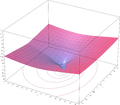$z = Re(W 0 (x + iy))$
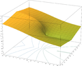$z = Im(W 0 (x + iy))$
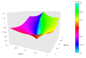
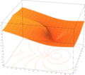$z = | W 0 (x + iy) |$
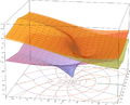Superimposition of the previous three plots

Numerical evaluation

The $W$ function may be approximated using Newton's method, with successive approximations to $w = W (z)$ (so $z = we w$ ) being

w_{j+1}=w_{j}-{\frac {w_{j}e^{w_{j}}-z}{e^{w_{j}}+w_{j}e^{w_{j}}}}.

The $W$ function may also be approximated using Halley's method,

w_{j+1}=w_{j}-{\frac {w_{j}e^{w_{j}}-z}{e^{w_{j}}\left(w_{j}+1\right)-{\dfrac {\left(w_{j}+2\right)\left(w_{j}e^{w_{j}}-z\right)}{2w_{j}+2}}}}

given in Corless et al.^[2] to compute $W$ .

Software

The Lambert $W$ function is implemented as LambertW in Maple, lambertw in GP (and glambertW in PARI), lambertw in Matlab,^[32] also lambertw in octave with the specfun package, as lambert_w in Maxima,^[33] as ProductLog (with a silent alias LambertW) in Mathematica,^[34] as lambertw in Python scipy's special function package,^[35] as LambertW in Perl's ntheory module,^[36] and as gsl_sf_lambert_W0 and gsl_sf_lambert_Wm1 functions in the special functions section of the GNU Scientific Library (GSL). In R, the Lambert $W$ function is implemented as the lambertW0 and lambertWm1 functions in the lamW package.^[37]

A C++ code for all the branches of the complex Lambert $W$ function is available on the homepage of István Mező.^[38]

Notes

↑ Chow, Timothy Y. (1999), "What is a closed-form number?", American Mathematical Monthly, 106 (5): 440–448, arXiv:math/9805045, doi:10.2307/2589148, JSTOR 2589148, MR 1699262 .
1 2 3 Corless, R. M.; Gonnet, G. H.; Hare, D. E. G.; Jeffrey, D. J.; Knuth, D. E. (1996). "On the Lambert W function" (PostScript). Advances in Computational Mathematics. 5: 329–359. doi:10.1007/BF02124750.
↑ Lambert J. H., "Observationes variae in mathesin puram", Acta Helveticae physico-mathematico-anatomico-botanico-medica, Band III, 128–168, 1758.
↑ Euler, L. "De serie Lambertina Plurimisque eius insignibus proprietatibus". Acta Acad. Scient. Petropol. 2, 29–51, 1783. Reprinted in Euler, L. Opera Omnia, Series Prima, Vol. 6: Commentationes Algebraicae. Leipzig, Germany: Teubner, pp. 350–369, 1921.
1 2 Corless, R. M.; Gonnet, G. H.; Hare, D. E. G.; Jeffrey, D. J. (1993). "Lambert's W function in Maple". The Maple Technical Newsletter. 9: 12–22. CiteSeerX 10.1.1.33.2556.
↑ Approximation of the Lambert W function and the hyperpower function, Hoorfar, Abdolhossein; Hassani, Mehdi.
↑ A. Hoorfar, M. Hassani, Inequalities on the Lambert W Function and Hyperpower Function, JIPAM, volume 9, issue 2, article 51. 2008.
↑ Chatzigeorgiou, I. (2013). "Bounds on the Lambert function and their Application to the Outage Analysis of User Cooperation". IEEE Communications Letters. 17 (8): 1505–1508. arXiv:1601.04895. doi:10.1109/LCOMM.2013.070113.130972.
↑ "Lambert function: Identities (formula 01.31.17.0001)".
↑ "Lambert W-Function".
↑ Finch, S. R. (2003). Mathematical constants. Cambridge University Press. p. 450.
↑ István, Mező. "An integral representation for the principal branch of Lambert the W function". Retrieved 7 November 2017.
↑ Dubinov, A. E.; Dubinova, I. D.; Saǐkov, S. K. (2006). The Lambert W Function and Its Applications to Mathematical Problems of Physics (in Russian). RFNC-VNIIEF. p. 53.
↑ Robert M., Corless; David J., Jeffrey; Donald E., Knuth (1997). A sequence of series for the Lambert W function. Proceedings of the 1997 International Symposium on Symbolic and Algebraic Computation. pp. 197–204. doi:10.1145/258726.258783. ISBN 978-0897918756.
↑ "The Lambert W Function". Ontario Research Centre.
↑ B Ohayon., G Ron. (2013). "New approaches in designing a Zeeman Slower". Journal of Instrumentation. 8 (2): P02016. arXiv:1212.2109. Bibcode:2013JInst...8P2016O. doi:10.1088/1748-0221/8/02/P02016.
↑ Sotero, Roberto C.; Iturria-Medina, Yasser (2011). "From Blood oxygenation level dependent (BOLD) signals to brain temperature maps". Bull Math Biol (Submitted manuscript). 73 (11): 2731–47. doi:10.1007/s11538-011-9645-5. PMID 21409512.
↑ Braun, Artur; Wokaun, Alexander; Hermanns, Heinz-Guenter (2003). "Analytical Solution to a Growth Problem with Two Moving Boundaries". Appl Math Model. 27 (1): 47–52. doi:10.1016/S0307-904X(02)00085-9.
↑ Braun, Artur; Baertsch, Martin; Schnyder, Bernhard; Koetz, Ruediger (2000). "A Model for the film growth in samples with two moving boundaries – An Application and Extension of the Unreacted-Core Model". Chem Eng Sci. 55 (22): 5273–5282. doi:10.1016/S0009-2509(00)00143-3.
↑ Braun, Artur; Briggs, Keith M.; Boeni, Peter (2003). "Analytical solution to Matthews' and Blakeslee's critical dislocation formation thickness of epitaxially grown thin films". J Cryst Growth. 241 (1–2): 231–234. Bibcode:2002JCrGr.241..231B. doi:10.1016/S0022-0248(02)00941-7.
↑ Colla, Pietro (2014). "A New Analytical Method for the Motion of a Two-Phase Interface in a Tilted Porous Medium". PROCEEDINGS,Thirty-Eighth Workshop on Geothermal Reservoir Engineering,Stanford University. SGP-TR-202. ()
↑ de la Madrid, R. (2017). "Numerical calculation of the decay widths, the decay constants, and the decay energy spectra of the resonances of the delta-shell potential". Nucl. Phys. A. 962: 24–45. arXiv:1704.00047. Bibcode:2017NuPhA.962...24D. doi:10.1016/j.nuclphysa.2017.03.006.
↑ Floratos, Emmanuel; Georgiou, George; Linardopoulos, Georgios (2014). "Large-Spin Expansions of GKP Strings". JHEP. 03 (3): 0180. arXiv:1311.5800. doi:10.1007/JHEP03(2014)018.
↑ Floratos, Emmanuel; Linardopoulos, Georgios (2015). "Large-Spin and Large-Winding Expansions of Giant Magnons and Single Spikes". Nucl. Phys. B. 897: 229–275. arXiv:1406.0796. doi:10.1016/j.nuclphysb.2015.05.021.
↑ Scott, T. C.; Mann, R. B.; Martinez Ii, Roberto E. (2006). "General Relativity and Quantum Mechanics: Towards a Generalization of the Lambert W Function". AAECC (Applicable Algebra in Engineering, Communication and Computing). 17 (1): 41–47. arXiv:math-ph/0607011. doi:10.1007/s00200-006-0196-1.
↑ Scott, T. C.; Fee, G.; Grotendorst, J. (2013). "Asymptotic series of Generalized Lambert W Function". SIGSAM (ACM Special Interest Group in Symbolic and Algebraic Manipulation). 47 (185): 75–83. doi:10.1145/2576802.2576804.
↑ Scott, T. C.; Fee, G.; Grotendorst, J.; Zhang, W.Z. (2014). "Numerics of the Generalized Lambert W Function". SIGSAM. 48 (1/2): 42–56. doi:10.1145/2644288.2644298.
↑ Farrugia, P. S.; Mann, R. B.; Scott, T. C. (2007). "N-body Gravity and the Schrödinger Equation". Class. Quantum Grav. 24 (18): 4647–4659. arXiv:gr-qc/0611144. Bibcode:2007CQGra..24.4647F. doi:10.1088/0264-9381/24/18/006.
↑ Scott, T. C.; Aubert-Frécon, M.; Grotendorst, J. (2006). "New Approach for the Electronic Energies of the Hydrogen Molecular Ion". Chem. Phys. 324 (2–3): 323–338. arXiv:physics/0607081. Bibcode:2006CP....324..323S. CiteSeerX 10.1.1.261.9067. doi:10.1016/j.chemphys.2005.10.031.
↑ Maignan, Aude; Scott, T. C. (2016). "Fleshing out the Generalized Lambert W Function". SIGSAM. 50 (2): 45–60. doi:10.1145/2992274.2992275.
↑ Scott, T. C.; Lüchow, A.; Bressanini, D.; Morgan, J. D. III (2007). "The Nodal Surfaces of Helium Atom Eigenfunctions". Phys. Rev. A. 75 (6): 060101. Bibcode:2007PhRvA..75f0101S. doi:10.1103/PhysRevA.75.060101.
↑ lambertw – MATLAB
↑ Maxima, a Computer Algebra System
↑ ProductLog at WolframAlpha
↑ "Scipy.special.lambertw — SciPy v0.16.1 Reference Guide".
↑ ntheory at MetaCPAN
↑ Adler, Avraham (2017-04-24), lamW: Lambert W Function, retrieved 2017-12-19
↑ The webpage of István Mező

References

Corless, R.; Gonnet, G.; Hare, D.; Jeffrey, D.; Knuth, Donald (1996). "On the Lambert W function" (PDF). Advances in Computational Mathematics. 5: 329–359. doi:10.1007/BF02124750. ISSN 1019-7168
Chapeau-Blondeau, F.; Monir, A. (2002). "Evaluation of the Lambert W Function and Application to Generation of Generalized Gaussian Noise With Exponent 1/2" (PDF). IEEE Trans. Signal Processing. 50 (9).
Francis; et al. (2000). "Quantitative General Theory for Periodic Breathing". Circulation. 102 (18): 2214–21. CiteSeerX 10.1.1.505.7194. doi:10.1161/01.cir.102.18.2214. PMID 11056095. (Lambert function is used to solve delay-differential dynamics in human disease.)
Hayes, B. (2005). "Why W?" (PDF). American Scientist. 93 (2): 104–108. doi:10.1511/2005.2.104.
Roy, R.; Olver, F. W. J. (2010), "Lambert W function", in Olver, Frank W. J.; Lozier, Daniel M.; Boisvert, Ronald F.; Clark, Charles W., NIST Handbook of Mathematical Functions, Cambridge University Press, ISBN 978-0521192255, MR 2723248
Stewart, Seán M. (2005). "A New Elementary Function for Our Curricula?" (PDF). Australian Senior Mathematics Journal. 19 (2): 8–26. ISSN 0819-4564. ERIC EJ720055. Lay summary.
Veberic, D., "Having Fun with Lambert W(x) Function" arXiv:1003.1628 (2010); Veberic, D. (2012). "Lambert W function for applications in physics". Computer Physics Communications. 183 (12): 2622–2628. arXiv:1209.0735. Bibcode:2012CoPhC.183.2622V. doi:10.1016/j.cpc.2012.07.008.
Chatzigeorgiou, I. (2013). "Bounds on the Lambert function and their Application to the Outage Analysis of User Cooperation". IEEE Communications Letters. 17 (8): 1505–1508. arXiv:1601.04895. doi:10.1109/LCOMM.2013.070113.130972.

External links

National Institute of Science and Technology Digital Library – Lambert W
MathWorld – Lambert W-Function
Computing the Lambert W function
Corless et al. Notes about Lambert W research
GPL C++ implementation with Halley's and Fritsch's iteration.
Special Functions of the GNU Scientific Library – GSL

This article is issued from Wikipedia. The text is licensed under Creative Commons - Attribution - Sharealike. Additional terms may apply for the media files.

[1] Chow, Timothy Y. (1999), "What is a closed-form number?", American Mathematical Monthly, 106 (5): 440–448, arXiv:math/9805045, doi:10.2307/2589148, JSTOR 2589148, MR 1699262 .

[Corless-2] 1 2 3 Corless, R. M.; Gonnet, G. H.; Hare, D. E. G.; Jeffrey, D. J.; Knuth, D. E. (1996). "On the Lambert W function" (PostScript). Advances in Computational Mathematics. 5: 329–359. doi:10.1007/BF02124750.

[3] Lambert J. H., "Observationes variae in mathesin puram", Acta Helveticae physico-mathematico-anatomico-botanico-medica, Band III, 128–168, 1758.

[4] Euler, L. "De serie Lambertina Plurimisque eius insignibus proprietatibus". Acta Acad. Scient. Petropol. 2, 29–51, 1783. Reprinted in Euler, L. Opera Omnia, Series Prima, Vol. 6: Commentationes Algebraicae. Leipzig, Germany: Teubner, pp. 350–369, 1921.

[corless_maple-5] 1 2 Corless, R. M.; Gonnet, G. H.; Hare, D. E. G.; Jeffrey, D. J. (1993). "Lambert's W function in Maple". The Maple Technical Newsletter. 9: 12–22. CiteSeerX 10.1.1.33.2556.

[6] Approximation of the Lambert W function and the hyperpower function, Hoorfar, Abdolhossein; Hassani, Mehdi.

[7] A. Hoorfar, M. Hassani, Inequalities on the Lambert W Function and Hyperpower Function, JIPAM, volume 9, issue 2, article 51. 2008.

[Chatzigeorgiou-8] Chatzigeorgiou, I. (2013). "Bounds on the Lambert function and their Application to the Outage Analysis of User Cooperation". IEEE Communications Letters. 17 (8): 1505–1508. arXiv:1601.04895. doi:10.1109/LCOMM.2013.070113.130972.

[9] "Lambert function: Identities (formula 01.31.17.0001)".

[10] "Lambert W-Function".

[Finch-11] Finch, S. R. (2003). Mathematical constants. Cambridge University Press. p. 450.

[12] István, Mező. "An integral representation for the principal branch of Lambert the W function". Retrieved 7 November 2017.

[Dubinov-13] Dubinov, A. E.; Dubinova, I. D.; Saǐkov, S. K. (2006). The Lambert W Function and Its Applications to Mathematical Problems of Physics (in Russian). RFNC-VNIIEF. p. 53.

[14] Robert M., Corless; David J., Jeffrey; Donald E., Knuth (1997). A sequence of series for the Lambert W function. Proceedings of the 1997 International Symposium on Symbolic and Algebraic Computation. pp. 197–204. doi:10.1145/258726.258783. ISBN 978-0897918756.

[15] "The Lambert W Function". Ontario Research Centre.

[16] B Ohayon., G Ron. (2013). "New approaches in designing a Zeeman Slower". Journal of Instrumentation. 8 (2): P02016. arXiv:1212.2109. Bibcode:2013JInst...8P2016O. doi:10.1088/1748-0221/8/02/P02016.

[17] Sotero, Roberto C.; Iturria-Medina, Yasser (2011). "From Blood oxygenation level dependent (BOLD) signals to brain temperature maps". Bull Math Biol (Submitted manuscript). 73 (11): 2731–47. doi:10.1007/s11538-011-9645-5. PMID 21409512.

[18] Braun, Artur; Wokaun, Alexander; Hermanns, Heinz-Guenter (2003). "Analytical Solution to a Growth Problem with Two Moving Boundaries". Appl Math Model. 27 (1): 47–52. doi:10.1016/S0307-904X(02)00085-9.

[19] Braun, Artur; Baertsch, Martin; Schnyder, Bernhard; Koetz, Ruediger (2000). "A Model for the film growth in samples with two moving boundaries – An Application and Extension of the Unreacted-Core Model". Chem Eng Sci. 55 (22): 5273–5282. doi:10.1016/S0009-2509(00)00143-3.

[20] Braun, Artur; Briggs, Keith M.; Boeni, Peter (2003). "Analytical solution to Matthews' and Blakeslee's critical dislocation formation thickness of epitaxially grown thin films". J Cryst Growth. 241 (1–2): 231–234. Bibcode:2002JCrGr.241..231B. doi:10.1016/S0022-0248(02)00941-7.

[21] Colla, Pietro (2014). "A New Analytical Method for the Motion of a Two-Phase Interface in a Tilted Porous Medium". PROCEEDINGS,Thirty-Eighth Workshop on Geothermal Reservoir Engineering,Stanford University. SGP-TR-202. ()

[22] Madrid, R. (2017). "Numerical calculation of the decay widths, the decay constants, and the decay energy spectra of the resonances of the delta-shell potential". Nucl. Phys. A. 962: 24–45. arXiv:1704.00047. Bibcode:2017NuPhA.962...24D. doi:10.1016/j.nuclphysa.2017.03.006.

[23] Floratos, Emmanuel; Georgiou, George; Linardopoulos, Georgios (2014). "Large-Spin Expansions of GKP Strings". JHEP. 03 (3): 0180. arXiv:1311.5800. doi:10.1007/JHEP03(2014)018.

[24] Floratos, Emmanuel; Linardopoulos, Georgios (2015). "Large-Spin and Large-Winding Expansions of Giant Magnons and Single Spikes". Nucl. Phys. B. 897: 229–275. arXiv:1406.0796. doi:10.1016/j.nuclphysb.2015.05.021.

[25] Scott, T. C.; Mann, R. B.; Martinez Ii, Roberto E. (2006). "General Relativity and Quantum Mechanics: Towards a Generalization of the Lambert W Function". AAECC (Applicable Algebra in Engineering, Communication and Computing). 17 (1): 41–47. arXiv:math-ph/0607011. doi:10.1007/s00200-006-0196-1.

[26] Scott, T. C.; Fee, G.; Grotendorst, J. (2013). "Asymptotic series of Generalized Lambert W Function". SIGSAM (ACM Special Interest Group in Symbolic and Algebraic Manipulation). 47 (185): 75–83. doi:10.1145/2576802.2576804.

[27] Scott, T. C.; Fee, G.; Grotendorst, J.; Zhang, W.Z. (2014). "Numerics of the Generalized Lambert W Function". SIGSAM. 48 (1/2): 42–56. doi:10.1145/2644288.2644298.

[28] Farrugia, P. S.; Mann, R. B.; Scott, T. C. (2007). "N-body Gravity and the Schrödinger Equation". Class. Quantum Grav. 24 (18): 4647–4659. arXiv:gr-qc/0611144. Bibcode:2007CQGra..24.4647F. doi:10.1088/0264-9381/24/18/006.

[29] Scott, T. C.; Aubert-Frécon, M.; Grotendorst, J. (2006). "New Approach for the Electronic Energies of the Hydrogen Molecular Ion". Chem. Phys. 324 (2–3): 323–338. arXiv:physics/0607081. Bibcode:2006CP....324..323S. CiteSeerX 10.1.1.261.9067. doi:10.1016/j.chemphys.2005.10.031.

[30] Maignan, Aude; Scott, T. C. (2016). "Fleshing out the Generalized Lambert W Function". SIGSAM. 50 (2): 45–60. doi:10.1145/2992274.2992275.

[31] Scott, T. C.; Lüchow, A.; Bressanini, D.; Morgan, J. D. III (2007). "The Nodal Surfaces of Helium Atom Eigenfunctions". Phys. Rev. A. 75 (6): 060101. Bibcode:2007PhRvA..75f0101S. doi:10.1103/PhysRevA.75.060101.

[32] rtw – MATLAB

[33] Maxima, a Computer Algebra System

[34] ProductLog at WolframAlpha

[35] "Scipy.special.lambertw — SciPy v0.16.1 Reference Guide".

[36] theory at MetaCPAN

[37] Adler, Avraham (2017-04-24), lamW: Lambert W Function, retrieved 2017-12-19

[38] The webpage of István Mező

Lambert ''W'' function

Terminology

History

Calculus

Derivative

Antiderivative

Asymptotic expansions

Integer and complex powers

Identities

Special values

Representations

Branches and range

Other formulas

Definite integrals

Indefinite integrals

Solutions of equations

Example 1

Example 2

Example 3

Example 4

Example 5

Example 6

Example 7

Applications

Instrument design

Viscous flows

Neuroimaging

Chemical engineering

Materials science

Porous media

Bernoulli numbers and Todd genus

Statistics

Exact solutions of the Schrödinger equation

Exact solutions of the Einstein vacuum equations

Resonances of the delta-shell potential

Thermodynamic equilibrium

AdS/CFT correspondence

Generalizations

Plots

Numerical evaluation

Software

See also

Notes

References

External links