Bernoulli number

Bernoulli numbers $B \pm n$
$n$	fraction	decimal
0	1	+1.000000000
1	±1/2	±0.500000000
2	1/6	+0.166666666
3	0	+0.000000000
4	−1/30	−0.033333333
5	0	+0.000000000
6	1/42	+0.023809523
7	0	+0.000000000
8	−1/30	−0.033333333
9	0	+0.000000000
10	5/66	+0.075757575
11	0	+0.000000000
12	−691/2730	−0.253113553
13	0	+0.000000000
14	7/6	+1.166666666
15	0	+0.000000000
16	−3617/510	−7.092156862
17	0	+0.000000000
18	43867/798	+54.97117794
19	0	+0.000000000
20	−174611/330	−529.1242424

Graphs of modern Bernoulli numbers,

B

(circles) compared with Bernoulli numbers in older literature,

B *

(crosses).^[1]

In mathematics, the Bernoulli numbers $B n$ are a sequence of rational numbers which occur frequently in number theory. The values of the first 20 Bernoulli numbers are given in the table to the right. For every even $n$ other than 0, $B n$ is negative if $n$ is divisible by 4 and positive otherwise. For every odd $n$ other than 1, $B n = 0$ .

The superscript ± used in this article designates the two sign conventions for Bernoulli numbers. Only the $n = 1$ term is affected:

$B - n$ with $B - 1 = - 1 / 2$ ( A027641 / A027642) is the sign convention prescribed by NIST and most modern textbooks.^[2]
$B + n$ with $B + 1 = + 1 / 2$ ( A164555 / A027642) is sometimes used in the older literature.^[3]

In the formulas below, one can switch from one sign convention to the other with the relation $B_{n}^{+{}}=(-1)^{n}B_{n}^{-{}}$ .

The Bernoulli numbers are special values of the Bernoulli polynomials $B_{n}(x)$ , with $B_{n}^{-{}}=B_{n}(0)$ and $B_{n}^{+}=B_{n}(1)$ .^[3]

Since $B n = 0$ for all odd $n > 1$ , and many formulas only involve even-index Bernoulli numbers, some authors write " $B n$ " to mean $B 2 n$ . This article does not follow this notation.

The Bernoulli numbers appear in the Taylor series expansions of the tangent and hyperbolic tangent functions, in Faulhaber's formula for the sum of powers of the first positive integers, in the Euler–Maclaurin formula, and in expressions for certain values of the Riemann zeta function.

The Bernoulli numbers were discovered around the same time by the Swiss mathematician Jacob Bernoulli, after whom they are named, and independently by Japanese mathematician Seki Kōwa. Seki's discovery was posthumously published in 1712^[4]^[5] in his work Katsuyo Sampo; Bernoulli's, also posthumously, in his Ars Conjectandi of 1713. Ada Lovelace's note G on the Analytical Engine from 1842 describes an algorithm for generating Bernoulli numbers with Babbage's machine.^[6] As a result, the Bernoulli numbers have the distinction of being the subject of the first published complex computer program.

History

Early history

The Bernoulli numbers are rooted in the early history of the computation of sums of integer powers, which have been of interest to mathematicians since antiquity.

A page from Seki Takakazu's Katsuyo Sampo (1712), tabulating binomial coefficients and Bernoulli numbers

Methods to calculate the sum of the first $n$ positive integers, the sum of the squares and of the cubes of the first $n$ positive integers were known, but there were no real 'formulas', only descriptions given entirely in words. Among the great mathematicians of antiquity to consider this problem were Pythagoras (c. 572–497 BCE, Greece), Archimedes (287–212 BCE, Italy), Aryabhata (b. 476, India), Abu Bakr al-Karaji (d. 1019, Persia) and Abu Ali al-Hasan ibn al-Hasan ibn al-Haytham (965–1039, Iraq).

During the late sixteenth and early seventeenth centuries mathematicians made significant progress. In the West Thomas Harriot (1560–1621) of England, Johann Faulhaber (1580–1635) of Germany, Pierre de Fermat (1601–1665) and fellow French mathematician Blaise Pascal (1623–1662) all played important roles.

Thomas Harriot seems to have been the first to derive and write formulas for sums of powers using symbolic notation, but even he calculated only up to the sum of the fourth powers. Johann Faulhaber gave formulas for sums of powers up to the 17th power in his 1631 Academia Algebrae, far higher than anyone before him, but he did not give a general formula.

Blaise Pascal in 1654 proved Pascal's identity relating the sums of the $p$ th powers of the first $n$ positive integers for $p = 0, 1, 2, \dots, k$ .

The Swiss mathematician Jakob Bernoulli (1654–1705) was the first to realize the existence of a single sequence of constants $B 0, B 1, B 2,\dots$ which provide a uniform formula for all sums of powers (Knuth 1993).

The joy Bernoulli experienced when he hit upon the pattern needed to compute quickly and easily the coefficients of his formula for the sum of the $c$ th powers for any positive integer $c$ can be seen from his comment. He wrote:

"With the help of this table, it took me less than half of a quarter of an hour to find that the tenth powers of the first 1000 numbers being added together will yield the sum 91,409,924,241,424,243,424,241,924,242,500."

Bernoulli's result was published posthumously in Ars Conjectandi in 1713. Seki Kōwa independently discovered the Bernoulli numbers and his result was published a year earlier, also posthumously, in 1712.^[4] However, Seki did not present his method as a formula based on a sequence of constants.

Bernoulli's formula for sums of powers is the most useful and generalizable formulation to date. The coefficients in Bernoulli's formula are now called Bernoulli numbers, following a suggestion of Abraham de Moivre.

Bernoulli's formula is sometimes called Faulhaber's formula after Johann Faulhaber who found remarkable ways to calculate sum of powers but never stated Bernoulli's formula. To call Bernoulli's formula Faulhaber's formula does injustice to Bernoulli and simultaneously hides the genius of Faulhaber as Faulhaber's formula is in fact more efficient than Bernoulli's formula. According to Knuth (Knuth 1993) a rigorous proof of Faulhaber's formula was first published by Carl Jacobi in 1834 (Jacobi 1834). Knuth's in-depth study of Faulhaber's formula concludes (the nonstandard notation on the LHS is explained further on):

"Faulhaber never discovered the Bernoulli numbers; i.e., he never realized that a single sequence of constants

B 0, B 1, B 2,

… would provide a uniform

\quad \sum n^{m}={\frac {1}{m+1}}\left(B_{0}n^{m+1}+{\binom {m+1}{1}}B_{1}^{+}n^{m}+{\binom {m+1}{2}}B_{2}n^{m-1}+\cdots +{\binom {m+1}{m}}B_{m}n\right)

or

\quad \sum n^{m}={\frac {1}{m+1}}\left(B_{0}n^{m+1}-{\binom {m+1}{1}}B_{1}^{-{}}n^{m}+{\binom {m+1}{2}}B_{2}n^{m-1}-\cdots +(-1)^{m}{\binom {m+1}{m}}B_{m}n\right)

for all sums of powers. He never mentioned, for example, the fact that almost half of the coefficients turned out to be zero after he had converted his formulas for

\sum n m

from polynomials in $N$ to polynomials in $n$ ." (Knuth 1993, p. 14)

Reconstruction of "Summae Potestatum"

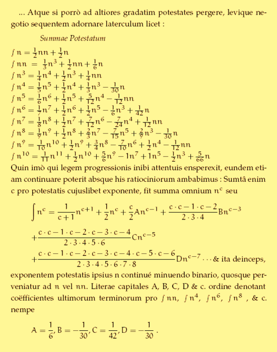
Jakob Bernoulli's "Summae Potestatum", 1713

The Bernoulli numbers A164555(n)/ A027642(n) were introduced by Jakob Bernoulli in the book Ars Conjectandi published posthumously in 1713 page 97. The main formula can be seen in the second half of the corresponding facsimile. The constant coefficients denoted $A$ , $B$ , $C$ and $D$ by Bernoulli are mapped to the notation which is now prevalent as $A = B 2$ , $B = B 4$ , $C = B 6$ , $D = B 8$ . The expression $c \cdot c -1\cdot c -2\cdot c -3$ means $c \cdot(c -1)\cdot(c -2)\cdot(c -3)$ – the small dots are used as grouping symbols. Using today's terminology these expressions are falling factorial powers $c k$ . The factorial notation $k!$ as a shortcut for $1 \times 2 \times \dots \times k$ was not introduced until 100 years later. The integral symbol on the left hand side goes back to Gottfried Wilhelm Leibniz in 1675 who used it as a long letter $S$ for "summa" (sum). (The Mathematics Genealogy Project^[7] shows Leibniz as the academic advisor of Jakob Bernoulli. See also the Earliest Uses of Symbols of Calculus.^[8]) The letter $n$ on the left hand side is not an index of summation but gives the upper limit of the range of summation which is to be understood as $1, 2, \dots, n$ . Putting things together, for positive $c$ , today a mathematician is likely to write Bernoulli's formula as:

\sum _{k=1}^{n}k^{c}={\frac {n^{c+1}}{c+1}}+{\frac {1}{2}}n^{c}+\sum _{k=2}^{c}{\frac {B_{k}}{k!}}c^{\underline {k-1}}n^{c-k+1}.

This formula suggests setting $B 1 = 1 / 2$ when switching from the so-called 'archaic' enumeration which uses only the even indices 2, 4, 6… to the modern form (more on different conventions in the next paragraph). Most striking in this context is the fact that the falling factorial $c k -1$ has for $k = 0$ the value $1 / c + 1$ .^[9] Thus Bernoulli's formula can be written

\sum _{k=1}^{n}k^{c}=\sum _{k=0}^{c}{\frac {B_{k}}{k!}}c^{\underline {k-1}}n^{c-k+1}

if $B 1 = 1/2$ , recapturing the value Bernoulli gave to the coefficient at that position.

Note that the formula for $\textstyle \sum _{k=1}^{n}k^{9}$ in the first half contains an error at the last term: it must be $-{\tfrac {3}{20}}n^{2}$ instead of $-{\tfrac {1}{12}}n^{2}$ .

Definitions

Many characterizations of the Bernoulli numbers have been found in the last 300 years, and each could be used to introduce these numbers. Here only three of the most useful ones are mentioned:

a recursive equation,
an explicit formula,
a generating function.

For the proof of the equivalence of the three approaches see (Ireland & Rosen 1990) or (Conway & Guy 1996).

Recursive definition

The Bernoulli numbers obey the sum formulas ^[3]

{\begin{aligned}\sum _{k=0}^{m}{\binom {m+1}{k}}B_{k}^{-{}}&=\delta _{m,0}\\\sum _{k=0}^{m}{\binom {m+1}{k}}B_{k}^{+{}}&=m+1\end{aligned}}

where $m=0,1,2...$ and $δ$ denotes the Kronecker delta. Solving for $B_{m}^{\mp {}}$ gives the recursive formulas

{\begin{aligned}B_{m}^{-{}}&=\delta _{m,0}-\sum _{k=0}^{m-1}{\binom {m}{k}}{\frac {B_{k}^{-{}}}{m-k+1}}\\B_{m}^{+}&=1-\sum _{k=0}^{m-1}{\binom {m}{k}}{\frac {B_{k}^{+}}{m-k+1}}\end{aligned}}

Explicit definition

In 1893 Louis Saalschütz listed a total of 38 explicit formulas for the Bernoulli numbers (Saalschütz 1893), usually giving some reference in the older literature. One of them is:

{\begin{aligned}B_{m}^{-{}}&=\sum _{k=0}^{m}\sum _{v=0}^{k}(-1)^{v}{\binom {k}{v}}{\frac {v^{m}}{k+1}}\\B_{m}^{+}&=\sum _{k=0}^{m}\sum _{v=0}^{k}(-1)^{v}{\binom {k}{v}}{\frac {(v+1)^{m}}{k+1}}.\end{aligned}}

Generating function

The exponential generating functions are

{\begin{aligned}{\frac {t}{e^{t}-1}}&={\frac {t}{2}}\left(\operatorname {coth} {\frac {t}{2}}-1\right)&=\sum _{m=0}^{\infty }{\frac {B_{m}^{-{}}t^{m}}{m!}}\\{\frac {t}{1-e^{-t}}}&={\frac {t}{2}}\left(\operatorname {coth} {\frac {t}{2}}+1\right)&=\sum _{m=0}^{\infty }{\frac {B_{m}^{+}t^{m}}{m!}}.\end{aligned}}

The (normal) generating function

z^{-1}\psi _{1}(z^{-1})=\sum _{m=0}^{\infty }B_{m}^{+}z^{m}

is an asymptotic series. It contains the trigamma function $ψ 1$ .

Bernoulli numbers and the Riemann zeta function

The Bernoulli numbers as given by the Riemann zeta function.

The Bernoulli numbers can be expressed in terms of the Riemann zeta function:

B + n = - nζ (1 - n)

for

n \geq 1

.

Here the argument of the zeta function is 0 or negative.

By means of the zeta functional equation and the gamma reflection formula the following relation can be obtained:^[10]

B_{2n}={\frac {(-1)^{n+1}2(2n)!}{(2\pi )^{2n}}}\zeta (2n)

for

n \geq 1

.

Now the argument of the zeta function is positive.

It then follows from $ζ \to 1$ ( $n \to \infty$ ) and Stirling's formula that

|B_{2n}|\sim 4{\sqrt {\pi n}}\left({\frac {n}{\pi e}}\right)^{2n}

for

n \to \infty

.

Efficient computation of Bernoulli numbers

In some applications it is useful to be able to compute the Bernoulli numbers $B 0$ through $B p - 3$ modulo $p$ , where $p$ is a prime; for example to test whether Vandiver's conjecture holds for $p$ , or even just to determine whether $p$ is an irregular prime. It is not feasible to carry out such a computation using the above recursive formulae, since at least (a constant multiple of) $p 2$ arithmetic operations would be required. Fortunately, faster methods have been developed (Buhler et al. 2001) which require only $O (p (log p) 2)$ operations (see big $O$ notation).

David Harvey (Harvey 2008) describes an algorithm for computing Bernoulli numbers by computing $B n$ modulo $p$ for many small primes $p$ , and then reconstructing $B n$ via the Chinese remainder theorem. Harvey writes that the asymptotic time complexity of this algorithm is $O (n 2 log(n) 2 + ε)$ and claims that this implementation is significantly faster than implementations based on other methods. Using this implementation Harvey computed $B n$ for $n = 10 8$ . Harvey's implementation has been included in SageMath since version 3.1. Prior to that, Bernd Kellner (Kellner 2002) computed $B n$ to full precision for $n = 10 6$ in December 2002 and Oleksandr Pavlyk (Pavlyk 2008) for $n = 10 7$ with Mathematica in April 2008.

Computer	Year	n	Digits*
J. Bernoulli	~1689	10	1
L. Euler	1748	30	8
J. C. Adams	1878	62	36
D. E. Knuth, T. J. Buckholtz	1967	7003167200000000000♠1672	7003333000000000000♠3330
G. Fee, S. Plouffe	1996	7004100000000000000♠10000	7004276770000000000♠27677
G. Fee, S. Plouffe	1996	7005100000000000000♠100000	7005376755000000000♠376755
B. C. Kellner	2002	7006100000000000000♠1000000	7006476752900000000♠4767529
O. Pavlyk	2008	7007100000000000000♠10000000	7007576752600000000♠57675260
D. Harvey	2008	7008100000000000000♠100000000	7008676752569000000♠676752569

* Digits is to be understood as the exponent of 10 when

B n

is written as a real number in normalized scientific notation.

Applications of the Bernoulli numbers

Asymptotic analysis

Arguably the most important application of the Bernoulli number in mathematics is their use in the Euler–Maclaurin formula. Assuming that $f$ is a sufficiently often differentiable function the Euler–Maclaurin formula can be written as ^[11]

\sum _{k=a}^{b-1}f(k)=\int _{a}^{b}f(x)\,dx+\sum _{k=1}^{m}{\frac {B_{k}^{-}}{k!}}(f^{(k-1)}(b)-f^{(k-1)}(a))+R_{-}(f,m).

This formulation assumes the convention $B - 1 = - 1 / 2$ . Using the convention $B + 1 = + 1 / 2$ the formula becomes

\sum _{k=a+1}^{b}f(k)=\int _{a}^{b}f(x)\,dx+\sum _{k=1}^{m}{\frac {B_{k}^{+}}{k!}}(f^{(k-1)}(b)-f^{(k-1)}(a))+R_{+}(f,m).

Here $f (0) = f$ (i.e. the zeroth-order derivative of a $f$ is just $f$ ). Moreover, let $f (-1)$ denote an antiderivative of $f$ . By the fundamental theorem of calculus,

\int _{a}^{b}f(x)\,dx=f^{(-1)}(b)-f^{(-1)}(a).

Thus the last formula can be further simplified to the following succinct form of the Euler–Maclaurin formula

\sum _{k=a}^{b}f(k)=\sum _{k=0}^{m}{\frac {B_{k}}{k!}}(f^{(k-1)}(b)-f^{(k-1)}(a))+R(f,m).

This form is for example the source for the important Euler–Maclaurin expansion of the zeta function

{\begin{aligned}\zeta (s)&=\sum _{k=0}^{m}{\frac {B_{k}^{+}}{k!}}s^{\overline {k-1}}+R(s,m)\\&={\frac {B_{0}}{0!}}s^{\overline {-1}}+{\frac {B_{1}^{+}}{1!}}s^{\overline {0}}+{\frac {B_{2}}{2!}}s^{\overline {1}}+\cdots +R(s,m)\\&={\frac {1}{s-1}}+{\frac {1}{2}}+{\frac {1}{12}}s+\cdots +R(s,m).\end{aligned}}

Here $s k$ denotes the rising factorial power.^[12]

Bernoulli numbers are also frequently used in other kinds of asymptotic expansions. The following example is the classical Poincaré-type asymptotic expansion of the digamma function $ψ$ .

\psi (z)\sim \ln z-\sum _{k=1}^{\infty }{\frac {B_{k}^{+}}{kz^{k}}}

Sum of powers

Bernoulli numbers feature prominently in the closed form expression of the sum of the $m$ th powers of the first $n$ positive integers. For $m, n \geq 0$ define

S_{m}(n)=\sum _{k=1}^{n}k^{m}=1^{m}+2^{m}+\cdots +n^{m}.

This expression can always be rewritten as a polynomial in $n$ of degree $m + 1$ . The coefficients of these polynomials are related to the Bernoulli numbers by Bernoulli's formula:

S_{m}(n)={\frac {1}{m+1}}\sum _{k=0}^{m}{\binom {m+1}{k}}B_{k}^{+}n^{m+1-k},

where $(m + 1 k)$ denotes the binomial coefficient.

For example, taking $m$ to be 1 gives the triangular numbers $0, 1, 3, 6, \dots$ A000217.

1+2+\cdots +n={\frac {1}{2}}(B_{0}n^{2}+2B_{1}^{+}n^{1})={\tfrac {1}{2}}(n^{2}+n).

Taking $m$ to be 2 gives the square pyramidal numbers $0, 1, 5, 14, \dots$ A000330.

1^{2}+2^{2}+\cdots +n^{2}={\frac {1}{3}}(B_{0}n^{3}+3B_{1}^{+}n^{2}+3B_{2}n^{1})={\tfrac {1}{3}}\left(n^{3}+{\tfrac {3}{2}}n^{2}+{\tfrac {1}{2}}n\right).

Some authors use the alternate convention for Bernoulli numbers and state Bernoulli's formula in this way:

S_{m}(n)={\frac {1}{m+1}}\sum _{k=0}^{m}(-1)^{k}{\binom {m+1}{k}}B_{k}^{-{}}n^{m+1-k}.

Bernoulli's formula is sometimes called Faulhaber's formula after Johann Faulhaber who also found remarkable ways to calculate sums of powers.

Faulhaber's formula was generalized by V. Guo and J. Zeng to a $q$ -analog (Guo & Zeng 2005).

Taylor series

The Bernoulli numbers appear in the Taylor series expansion of many trigonometric functions and hyperbolic functions.

Tangent: ${\begin{aligned}\tan x&=\sum _{n=1}^{\infty }{\frac {(-1)^{n-1}2^{2n}(2^{2n}-1)B_{2n}}{(2n)!}}\;x^{2n-1},&\left|x\right|&<{\frac {\pi }{2}}\\\end{aligned}}$

Cotangent: ${\begin{aligned}\cot x&{}={\frac {1}{x}}\sum _{n=0}^{\infty }{\frac {(-1)^{n}B_{2n}(2x)^{2n}}{(2n)!}},&\qquad 0<|x|<\pi .\end{aligned}}$

Hyperbolic tangent: ${\begin{aligned}\tanh x&=\sum _{n=1}^{\infty }{\frac {2^{2n}(2^{2n}-1)B_{2n}}{(2n)!}}\;x^{2n-1},&|x|&<{\frac {\pi }{2}}.\end{aligned}}$

Hyperbolic cotangent: ${\begin{aligned}\coth x&{}={\frac {1}{x}}\sum _{n=0}^{\infty }{\frac {B_{2n}(2x)^{2n}}{(2n)!}},&\qquad \qquad 0<|x|<\pi .\end{aligned}}$

Laurent series

The Bernoulli numbers appear in the following Laurent series:

Digamma function: $\psi (z)=\ln z-\sum _{k=1}^{\infty }{\frac {B_{k}^{+{}}}{kz^{k}}}$ ^[13]

Use in topology

The Kervaire–Milnor's formula for the order of the cyclic group of diffeomorphism classes of exotic $(4 n - 1)$ -spheres which bound parallelizable manifolds involves Bernoulli numbers. Let $ES n$ be the number of such exotic spheres for $n \geq 2$ , then

{\textit {ES}}_{n}=(2^{2n-2}-2^{4n-3})\operatorname {Numerator} \left({\frac {B_{4n}}{4n}}\right).

The Hirzebruch signature theorem for the $L$ genus of a smooth oriented closed manifold of dimension 4n also involves Bernoulli numbers.

Connections with combinatorial numbers

The connection of the Bernoulli number to various kinds of combinatorial numbers is based on the classical theory of finite differences and on the combinatorial interpretation of the Bernoulli numbers as an instance of a fundamental combinatorial principle, the inclusion–exclusion principle.

Connection with Worpitzky numbers

The definition to proceed with was developed by Julius Worpitzky in 1883. Besides elementary arithmetic only the factorial function $n!$ and the power function $k m$ is employed. The signless Worpitzky numbers are defined as

W_{n,k}=\sum _{v=0}^{k}(-1)^{v+k}(v+1)^{n}{\frac {k!}{v!(k-v)!}}.

They can also be expressed through the Stirling numbers of the second kind

W_{n,k}=k! \left\{ {n+1\atop k+1} \right\}.

A Bernoulli number is then introduced as an inclusion–exclusion sum of Worpitzky numbers weighted by the harmonic sequence 1, 1/2, 1/3, …

B_{n}=\sum _{k=0}^{n}(-1)^{k}{\frac {W_{n,k}}{k+1}}\ =\ \sum _{k=0}^{n}{\frac {1}{k+1}}\sum _{v=0}^{k}(-1)^{v}(v+1)^{n}{k \choose v}\ .

B 0 = 1

B 1 = 1 - 1 / 2

B 2 = 1 - 3 / 2 + 2 / 3

B 3 = 1 - 7 / 2 + 12 / 3 - 6 / 4

B 4 = 1 - 15 / 2 + 50 / 3 - 60 / 4 + 24 / 5

B 5 = 1 - 31 / 2 + 180 / 3 - 390 / 4 + 360 / 5 - 120 / 6

B 6 = 1 - 63 / 2 + 602 / 3 - 2100 / 4 + 3360 / 5 - 2520 / 6 + 720 / 7

This representation has $B + 1 = + 1 / 2$ .

Consider the sequence $s n$ , $n \geq 0$ . From Worpitzky's numbers A028246, A163626 applied to $s 0, s 0, s 1, s 0, s 1, s 2, s 0, s 1, s 2, s 3, \dots$ is identical to the Akiyama–Tanigawa transform applied to $s n$ (see Connection with Stirling numbers of the first kind). This can be seen via the table:

**Identity of Worpitzky's representation and Akiyama–Tanigawa transform**
1					0	1				0	0	1			0	0	0	1		0	0	0	0	1
1	−1				0	2	−2			0	0	3	−3		0	0	0	4	−4
1	−3	2			0	4	−10	6		0	0	9	−21	12
1	−7	12	−6		0	8	−38	54	−24
1	−15	50	−60	24

The first row represents $s 0, s 1, s 2, s 3, s 4$ .

Hence for the second fractional Euler numbers A198631 ( $n$ ) / A006519 ( $n + 1$ ):

E 0 = 1

E 1 = 1 - 1 / 2

E 2 = 1 - 3 / 2 + 2 / 4

E 3 = 1 - 7 / 2 + 12 / 4 - 6 / 8

E 4 = 1 - 15 / 2 + 50 / 4 - 60 / 8 + 24 / 16

E 5 = 1 - 31 / 2 + 180 / 4 - 390 / 8 + 360 / 16 - 120 / 32

E 6 = 1 - 63 / 2 + 602 / 4 - 2100 / 8 + 3360 / 16 - 2520 / 32 + 720 / 64

A second formula representing the Bernoulli numbers by the Worpitzky numbers is for $n \geq 1$

B_{n}={\frac {n}{2^{n+1}-2}}\sum _{k=0}^{n-1}(-2)^{-k}\,W_{n-1,k}.

The simplified second Worpitzky's representation of the second Bernoulli numbers is:

A164555 ( $n + 1$ ) / A027642( $n + 1$ ) = $n + 1 / 2 n + 2 - 2$ × A198631( $n$ ) / A006519( $n + 1$ )

which links the second Bernoulli numbers to the second fractional Euler numbers. The beginning is:

1 / 2, 1 / 6, 0, - 1 / 30, 0, 1 / 42, \dots = (1 / 2, 1 / 3, 3 / 14, 2 / 15, 5 / 62, 1 / 21, \dots) \times (1, 1 / 2, 0, - 1 / 4, 0, 1 / 2, \dots)

The numerators of the first parentheses are A111701 (see Connection with Stirling numbers of the first kind).

Connection with Stirling numbers of the second kind

If $S (k, m)$ denotes Stirling numbers of the second kind^[14] then one has:

j^{k}=\sum _{m=0}^{k}{j^{\underline {m}}}S(k,m)

where $j m$ denotes the falling factorial.

If one defines the Bernoulli polynomials $B k (j)$ as:^[15]

B_{k}(j)=k\sum _{m=0}^{k-1}{\binom {j}{m+1}}S(k-1,m)m!+B_{k}

where $B k$ for $k = 0, 1, 2,\dots$ are the Bernoulli numbers.

Then after the following property of binomial coefficient:

{\binom {j}{m}}={\binom {j+1}{m+1}}-{\binom {j}{m+1}}

one has,

j^{k}={\frac {B_{k+1}(j+1)-B_{k+1}(j)}{k+1}}.

One also has following for Bernoulli polynomials,^[15]

B_{k}(j)=\sum _{n=0}^{k}{\binom {k}{n}}B_{n}j^{k-n}.

The coefficient of $j$ in $(j m + 1)$ is $(-1) m / m + 1$ .

Comparing the coefficient of $j$ in the two expressions of Bernoulli polynomials, one has:

B_{k}=\sum _{m=0}^{k}(-1)^{m}{\frac {m!}{m+1}}S(k,m)

(resulting in $B 1 = + 1 / 2$ ) which is an explicit formula for Bernoulli numbers and can be used to prove Von-Staudt Clausen theorem.^[16]^[17]^[18]

Connection with Stirling numbers of the first kind

The two main formulas relating the unsigned Stirling numbers of the first kind $[n m]$ to the Bernoulli numbers (with $B 1 = + 1 / 2$ ) are

\frac{1}{m!}\sum_{k=0}^m (-1)^{k} \left[{m+1\atop k+1}\right] B_k = \frac{1}{m+1},

and the inversion of this sum (for $n \geq 0$ , $m \geq 0$ )

{\frac {1}{m!}}\sum _{k=0}^{m}(-1)^{k}\left[{m+1 \atop k+1}\right]B_{n+k}=A_{n,m}.

Here the number $A n, m$ are the rational Akiyama–Tanigawa numbers, the first few of which are displayed in the following table.

Akiyama–Tanigawa number
$m$ $n$	0	1	2	3	4
0	1	1/2	1/3	1/4	1/5
1	1/2	1/3	1/4	1/5	…
2	1/6	1/6	3/20	…	…
3	0	1/30	…	…	…
4	−1/30	…	…	…	…

The Akiyama–Tanigawa numbers satisfy a simple recurrence relation which can be exploited to iteratively compute the Bernoulli numbers. This leads to the algorithm shown in the section 'algorithmic description' above. See A051714/ A051715.

An autosequence is a sequence which has its inverse binomial transform equal to the signed sequence. If the main diagonal is zeroes = A000004, the autosequence is of the first kind. Example: A000045, the Fibonacci numbers. If the main diagonal is the first upper diagonal multiplied by 2, it is of the second kind. Example: A164555/ A027642, the second Bernoulli numbers (see A190339). The Akiyama–Tanigawa transform applied to $2 - n$ = 1/ A000079 leads to A198631 (n) / A06519 (n + 1). Hence:

Akiyama–Tanigawa transform for the second Euler numbers
$m$ $n$	0	1	2	3	4
0	1	1/2	1/4	1/8	1/16
1	1/2	1/2	3/8	1/4	…
2	0	1/4	3/8	…	…
3	−1/4	−1/4	…	…	…
4	0	…	…	…	…

See A209308 and A227577. A198631 ( $n$ ) / A006519 ( $n + 1$ ) are the second (fractional) Euler numbers and an autosequence of the second kind.

(

A164555 (

n + 2

)/

A027642 (

n + 2

) =

1 / 6, 0, - 1 / 30, 0, 1 / 42, \dots

) × (

2 n + 3 - 2 / n + 2

=

3, 14 / 3, 15 / 2, 62 / 5, 21, \dots

) =

A198631 (

n + 1

)/

A006519 (

n + 2

) =

1 / 2, 0, - 1 / 4, 0, 1 / 2, \dots

.

Also valuable for A027641 / A027642 (see Connection with Worpitzky numbers).

Connection with Pascal’s triangle

There are formulas connecting Pascal's triangle to Bernoulli numbers ^[19]

B_{n}^{+}={\frac {|A_{n}|}{(n+1)!}}~~~

where $|A_{n}|$ is the determinant of a n-by-n square matrix part of Pascal’s triangle whose elements are: $a_{i,k}={\begin{cases}0&{\text{if }}k>1+i\\{i+1 \choose k-1}&{\text{otherwise}}\end{cases}}$

Example:

B_{6}^{+}={\frac {\det {\begin{pmatrix}1&2&0&0&0&0\\1&3&3&0&0&0\\1&4&6&4&0&0\\1&5&10&10&5&0\\1&6&15&20&15&6\\1&7&21&35&35&21\end{pmatrix}}}{7!}}={\frac {120}{5040}}={\frac {1}{42}}

Connection with Eulerian numbers

There are formulas connecting Eulerian numbers $⟨ n m ⟩$ to Bernoulli numbers:

{\begin{aligned}\sum _{m=0}^{n}(-1)^{m}\left\langle {n \atop m}\right\rangle &=2^{n+1}(2^{n+1}-1){\frac {B_{n+1}}{n+1}},\\\sum _{m=0}^{n}(-1)^{m}\left\langle {n \atop m}\right\rangle {\binom {n}{m}}^{-1}&=(n+1)B_{n}.\end{aligned}}

Both formulae are valid for $n \geq 0$ if $B 1$ is set to 1/2. If $B 1$ is set to −1/2 they are valid only for $n \geq 1$ and $n \geq 2$ respectively.

A binary tree representation

The Stirling polynomials $σ n (x)$ are related to the Bernoulli numbers by $B n = n! σ n (1)$ . S. C. Woon (Woon 1997) described an algorithm to compute $σ n (1)$ as a binary tree:

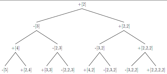
Woon's recursive algorithm (for $n \geq 1$ ) starts by assigning to the root node $N = [1,2]$ . Given a node $N = [a 1, a 2, \dots, a k]$ of the tree, the left child of the node is $L (N) = [- a 1, a 2 + 1, a 3, \dots, a k]$ and the right child $R (N) = [a 1, 2, a 2, \dots, a k]$ . A node $N = [a 1, a 2, \dots, a k]$ is written as $\pm[a 2, \dots, a k]$ in the initial part of the tree represented above with ± denoting the sign of $a 1$ .

Given a node $N$ the factorial of $N$ is defined as

N!=a_{1}\prod _{k=2}^{\operatorname {length} (N)}a_{k}!.

Restricted to the nodes $N$ of a fixed tree-level $n$ the sum of $1 / N!$ is $σ n (1)$ , thus

B_{n}=\sum _{\stackrel {N{\text{ node of}}}{{\text{ tree-level }}n}}{\frac {n!}{N!}}.

For example:

B 1 = 1!(1 / 2!)

B 2 = 2!(- 1 / 3! + 1 / 2!2!)

B 3 = 3!(1 / 4! - 1 / 2!3! - 1 / 3!2! + 1 / 2!2!2!)

Integral representation and continuation

The integral

b(s)=2e^{si\pi /2}\int _{0}^{\infty }{\frac {st^{s}}{1-e^{2\pi t}}}{\frac {dt}{t}}

has as special values $b (2 n) = B 2 n$ for $n > 0$ .

For example, $b (3) = 3 / 2 ζ (3) π -3 i$ and $b (5) = - 15 / 2 ζ (5) π -5 i$ . Here, $ζ$ is the Riemann zeta function, and $i$ is the imaginary unit. Leonhard Euler (Opera Omnia, Ser. 1, Vol. 10, p. 351) considered these numbers and calculated

{\begin{aligned}p&={\frac {3}{2\pi ^{3}}}\left(1+{\frac {1}{2^{3}}}+{\frac {1}{3^{3}}}+\cdots \right)=0.0581522\ldots \\q&={\frac {15}{2\pi ^{5}}}\left(1+{\frac {1}{2^{5}}}+{\frac {1}{3^{5}}}+\cdots \right)=0.0254132\ldots \end{aligned}}

The relation to the Euler numbers and $π$

The Euler numbers are a sequence of integers intimately connected with the Bernoulli numbers. Comparing the asymptotic expansions of the Bernoulli and the Euler numbers shows that the Euler numbers $E 2 n$ are in magnitude approximately $2 / π (4 2 n - 2 2 n)$ times larger than the Bernoulli numbers $B 2 n$ . In consequence:

\pi \sim 2(2^{2n}-4^{2n}){\frac {B_{2n}}{E_{2n}}}.

This asymptotic equation reveals that $π$ lies in the common root of both the Bernoulli and the Euler numbers. In fact $π$ could be computed from these rational approximations.

Bernoulli numbers can be expressed through the Euler numbers and vice versa. Since, for odd $n$ , $B n = E n = 0$ (with the exception $B 1$ ), it suffices to consider the case when $n$ is even.

{\begin{aligned}B_{n}&=\sum _{k=0}^{n-1}{\binom {n-1}{k}}{\frac {n}{4^{n}-2^{n}}}E_{k}&n&=2,4,6,\ldots \\E_{n}&=\sum _{k=1}^{n}{\binom {n}{k-1}}{\frac {2^{k}-4^{k}}{k}}B_{k}&n&=2,4,6,\ldots \end{aligned}}

These conversion formulas express an inverse relation between the Bernoulli and the Euler numbers. But more important, there is a deep arithmetic root common to both kinds of numbers, which can be expressed through a more fundamental sequence of numbers, also closely tied to $π$ . These numbers are defined for $n > 1$ as

S_{n}=2\left({\frac {2}{\pi }}\right)^{n}\sum _{k=-\infty }^{\infty }(4k+1)^{-n}\qquad k=0,-1,1,-2,2,\ldots

and $S 1 = 1$ by convention (Elkies 2003). The magic of these numbers lies in the fact that they turn out to be rational numbers. This was first proved by Leonhard Euler in a landmark paper (Euler 1735) ‘De summis serierum reciprocarum’ (On the sums of series of reciprocals) and has fascinated mathematicians ever since. The first few of these numbers are

S_n = 1,1,\frac{1}{2},\frac{1}{3},\frac{5}{24}, \frac{2}{15},\frac{61}{720},\frac{17}{315},\frac{277}{8064},\frac{62}{2835},\ldots

(

A099612 /

A099617)

These are the coefficients in the expansion of $sec x + tan x$ .

The Bernoulli numbers and Euler numbers are best understood as special views of these numbers, selected from the sequence $S n$ and scaled for use in special applications.

{\begin{aligned}B_{n}&=(-1)^{\left\lfloor {\frac {n}{2}}\right\rfloor }[n{\text{ even}}]{\frac {n!}{2^{n}-4^{n}}}\,S_{n}\ ,&n&=2,3,\ldots \\E_{n}&=(-1)^{\left\lfloor {\frac {n}{2}}\right\rfloor }[n{\text{ even}}]n!\,S_{n+1}&n&=0,1,\ldots \end{aligned}}

The expression [ $n$ even] has the value 1 if $n$ is even and 0 otherwise (Iverson bracket).

These identities show that the quotient of Bernoulli and Euler numbers at the beginning of this section is just the special case of $R n = 2 S n / S n + 1$ when $n$ is even. The $R n$ are rational approximations to $π$ and two successive terms always enclose the true value of $π$ . Beginning with $n = 1$ the sequence starts ( A132049 / A132050):

2, 4, 3, \frac{16}{5}, \frac{25}{8}, \frac{192}{61}, \frac{427}{136}, \frac{4352}{1385}, \frac{12465}{3968}, \frac{158720}{50521},\ldots \quad \longrightarrow \pi.

These rational numbers also appear in the last paragraph of Euler's paper cited above.

Consider the Akiyama–Tanigawa transform for the sequence A046978 ( $n + 2$ ) / A016116 ( $n + 1$ ):

0	1	1/2	0	−1/4	−1/4	−1/8	0
1	1/2	1	3/4	0	−5/8	−3/4
2	−1/2	1/2	9/4	5/2	5/8
3	−1	−7/2	−3/4	15/2
4	5/2	−11/2	−99/4
5	8	77/2
6	−61/2

From the second, the numerators of the first column are the denominators of Euler's formula. The first column is −1/2 × A163982.

An algorithmic view: the Seidel triangle

The sequence S_n has another unexpected yet important property: The denominators of S_n divide the factorial (n − 1)!. In other words: the numbers T_n = S_n(n − 1)!, sometimes called Euler zigzag numbers, are integers.

T_{n}=1,\,1,\,1,\,2,\,5,\,16,\,61,\,272,\,1385,\,7936,\,50521,\,353792,\ldots \quad n=0,1,2,3,\ldots

(

A000111). See (

A253671).

Thus the above representations of the Bernoulli and Euler numbers can be rewritten in terms of this sequence as

{\begin{aligned}B_{n}&=(-1)^{\left\lfloor {\frac {n}{2}}\right\rfloor }[n{\text{ even}}]{\frac {n}{2^{n}-4^{n}}}\,T_{n-1}\ &n&=2,3,\ldots \\E_{n}&=(-1)^{\left\lfloor {\frac {n}{2}}\right\rfloor }[n{\text{ even}}]T_{n+1}&n&=0,1,\ldots \end{aligned}}

These identities make it easy to compute the Bernoulli and Euler numbers: the Euler numbers $E n$ are given immediately by $T 2 n + 1$ and the Bernoulli numbers $B 2 n$ are obtained from $T 2 n$ by some easy shifting, avoiding rational arithmetic.

What remains is to find a convenient way to compute the numbers $T n$ . However, already in 1877 Philipp Ludwig von Seidel (Seidel 1877) published an ingenious algorithm which makes it extremely simple to calculate $T n$ .

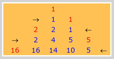
Start by putting 1 in row 0 and let $k$ denote the number of the row currently being filled
If $k$ is odd, then put the number on the left end of the row $k - 1$ in the first position of the row $k$ , and fill the row from the left to the right, with every entry being the sum of the number to the left and the number to the upper
At the end of the row duplicate the last number.
If $k$ is even, proceed similar in the other direction.

Seidel's algorithm is in fact much more general (see the exposition of Dominique Dumont (Dumont 1981)) and was rediscovered several times thereafter.

Similar to Seidel's approach D. E. Knuth and T. J. Buckholtz (Knuth & Buckholtz 1967) gave a recurrence equation for the numbers $T 2 n$ and recommended this method for computing $B 2 n$ and $E 2 n$ ‘on electronic computers using only simple operations on integers’.

V. I. Arnold rediscovered Seidel's algorithm in (Arnold 1991) and later Millar, Sloane and Young popularized Seidel's algorithm under the name boustrophedon transform.

Triangular form:

						1
					1		1
				2		2		1
			2		4		5		5
		16		16		14		10		5
	16		32		46		56		61		61
272		272		256		224		178		122		61

Only A000657, with one 1, and A214267, with two 1s, are in the OEIS.

Distribution with a supplementary 1 and one 0 in the following rows:

						1
					0		1
				−1		−1		0
			0		−1		−2		−2
		5		5		4		2		0
	0		5		10		14		16		16
−61		−61		−56		−46		−32		−16		0

This is A239005, a signed version of A008280. The main andiagonal is A122045. The main diagonal is A155585. The central column is A099023. Row sums: 1, 1, −2, −5, 16, 61…. See A163747. See the array beginning with 1, 1, 0, −2, 0, 16, 0 below.

The Akiyama–Tanigawa algorithm applied to A046978 ( $n + 1$ ) / A016116( $n$ ) yields:

1	1	1/2	0	−1/4	−1/4	−1/8
0	1	3/2	1	0	−3/4
−1	−1	3/2	4	15/4
0	−5	−15/2	1
5	5	−51/2
0	61
−61

1. The first column is A122045. Its binomial transform leads to:

1	1	0	−2	0	16	0
0	−1	−2	2	16	−16
−1	−1	4	14	−32
0	5	10	−46
5	5	−56
0	−61
−61

The first row of this array is A155585. The absolute values of the increasing antidiagonals are A008280. The sum of the antidiagonals is − A163747 ( $n + 1$ ).

2. The second column is 1 1 −1 −5 5 61 −61 −1385 1385…. Its binomial transform yields:

1	2	2	−4	−16	32	272
1	0	−6	−12	48	240
−1	−6	−6	60	192
−5	0	66	32
5	66	66
61	0
−61

The first row of this array is 1 2 2 −4 −16 32 272 544 −7936 15872 353792 −707584…. The absolute values of the second bisection are the double of the absolute values of the first bisection.

Consider the Akiyama-Tanigawa algorithm applied to A046978 ( $n$ ) / ( A158780 ( $n + 1$ ) = abs( A117575 ( $n$ )) + 1 = 1, 2, 2, 3/2, 1, 3/4, 3/4, 7/8, 1, 17/16, 17/16, 33/32….

1	2	2	3/2	1	3/4	3/4
−1	0	3/2	2	5/4	0
−1	−3	−3/2	3	25/4
2	−3	−27/2	−13
5	21	−3/2
−16	45
−61

The first column whose the absolute values are A000111 could be the numerator of a trigonometric function.

A163747 is an autosequence of the first kind (the main diagonal is A000004). The corresponding array is:

0	−1	−1	2	5	−16	−61
−1	0	3	3	−21	−45
1	3	0	−24	−24
2	−3	−24	0
−5	−21	24
−16	45
−61

The first two upper diagonals are −1 3 −24 402… = $(-1) n + 1$ × A002832. The sum of the antidiagonals is 0 −2 0 10… = 2 × A122045(n + 1).

− A163982 is an autosequence of the second kind, like for instance A164555 / A027642. Hence the array:

2	1	−1	−2	5	16	−61
−1	−2	−1	7	11	−77
−1	1	8	4	−88
2	7	−4	−92
5	−11	−88
−16	−77
−61

The main diagonal, here 2 −2 8 −92…, is the double of the first upper one, here A099023. The sum of the antidiagonals is 2 0 −4 0… = 2 × A155585( $n +$ 1). Note that A163747 − A163982 = 2 × A122045.

A combinatorial view: alternating permutations

Around 1880, three years after the publication of Seidel's algorithm, Désiré André proved a now classic result of combinatorial analysis (André 1879) & (André 1881). Looking at the first terms of the Taylor expansion of the trigonometric functions $tan x$ and $sec x$ André made a startling discovery.

{\begin{aligned}\tan x&=x+{\frac {2x^{3}}{3!}}+{\frac {16x^{5}}{5!}}+{\frac {272x^{7}}{7!}}+{\frac {7936x^{9}}{9!}}+\cdots \\[6pt]\sec x&=1+{\frac {x^{2}}{2!}}+{\frac {5x^{4}}{4!}}+{\frac {61x^{6}}{6!}}+{\frac {1385x^{8}}{8!}}+{\frac {50521x^{10}}{10!}}+\cdots \end{aligned}}

The coefficients are the Euler numbers of odd and even index, respectively. In consequence the ordinary expansion of $tan x + sec x$ has as coefficients the rational numbers $S n$ .

\tan x+\sec x=1+x+{\tfrac {1}{2}}x^{2}+{\tfrac {1}{3}}x^{3}+{\tfrac {5}{24}}x^{4}+{\tfrac {2}{15}}x^{5}+{\tfrac {61}{720}}x^{6}+\cdots

André then succeeded by means of a recurrence argument to show that the alternating permutations of odd size are enumerated by the Euler numbers of odd index (also called tangent numbers) and the alternating permutations of even size by the Euler numbers of even index (also called secant numbers).

Related sequences

The arithmetic mean of the first and the second Bernoulli numbers are the associate Bernoulli numbers: $B 0 = 1$ , $B 1 = 0$ , $B 2 = 1 / 6$ , $B 3 = 0$ , $B 4 = - 1 / 30$ , A176327 / A027642. Via the second row of its inverse Akiyama–Tanigawa transform A177427, they lead to Balmer series A061037 / A061038.

The Akiyama–Tanigawa algorithm applied to A060819 ( $n + 4$ ) / A145979 ( $n$ ) leads to the Bernoulli numbers A027641 / A027642, A164555 / A027642, or A176327 A176289 without $B 1$ , named intrinsic Bernoulli numbers $B i (n)$ .

1	5/6	3/4	7/10	2/3
1/6	1/6	3/20	2/15	5/42
0	1/30	1/20	2/35	5/84
−1/30	−1/30	−3/140	−1/105	0
0	−1/42	−1/28	−4/105	−1/28

Hence another link between the intrinsic Bernoulli numbers and the Balmer series via A145979 ( $n$ ).

A145979 ( $n - 2$ ) = 0, 2, 1, 6,… is a permutation of the non-negative numbers.

The terms of the first row are f(n) = $1 / 2 + 1 / n + 2$ . 2, f(n) is an autosequence of the second kind. 3/2, f(n) leads by its inverse binomial transform to 3/2 −1/2 1/3 −1/4 1/5 ... = 1/2 + log 2.

Consider g(n) = 1/2 - 1 / (n+2) = 0, 1/6, 1/4, 3/10, 1/3. The Akiyama-Tanagiwa transforms gives:

0	1/6	1/4	3/10	1/3	5/14	...
−1/6	−1/6	−3/20	−2/15	−5/42	−3/28	...
0	−1/30	−1/20	−2/35	−5/84	−5/84	...
1/30	1/30	3/140	1/105	0	−1/140	...

0, g(n), is an autosequence of the second kind.

Euler A198631 ( $n$ ) / A006519 ( $n + 1$ ) without the second term (1/2) are the fractional intrinsic Euler numbers $E i (n) = 1, 0, - 1 / 4, 0, 1 / 2, 0, - 17 / 8, 0, \dots$ The corresponding Akiyama transform is:

1	1	7/8	3/4	21/32
0	1/4	3/8	3/8	5/16
−1/4	−1/4	0	1/4	25/64
0	−1/2	−3/4	−9/16	−5/32
1/2	1/2	−9/16	−13/8	−125/64

The first line is $Eu (n)$ . $Eu (n)$ preceded by a zero is an autosequence of the first kind. It is linked to the Oresme numbers. The numerators of the second line are A069834 preceded by 0. The difference table is:

0	1	1	7/8	3/4	21/32	19/32
1	0	−1/8	−1/8	−3/32	−1/16	−5/128
−1	−1/8	0	1/32	1/32	3/128	1/64

Generalization to the odd-index Bernoulli numbers

The Bernoulli numbers $B n$ for n = 0, 1, 2, 3, ... are

1, 1/2, 1/6, 3/56, 1/30, 25/992, 1/42, 427/16256, 1/30, 12465/261632, 5/66, 555731/4102256, 691/2730, 35135945/67100672, 7/6, 2990414715/1073709056, ... (

A193472/

A193473)^[20]

This is $ez (n - 1) n! / 4 n - 2 n$ where $ez (n)$ is the $n$ th coefficient of $sec t + tan t$ ( A000111/ A000142).

A companion to the Bernoulli numbers

See A190339. The following fractional numbers are an autosequence of the first kind.

A191754 /

A192366 = 0, 1/2, 1/2, 1/3, 1/6, 1/15, 1/30, 1/35, 1/70, –1/105, –1/210, 41/1155, 41/2310, –589/5005, −589/10010 …

Apply $T (n + 1, k) = 2 T (n, k + 1) - T (n, k) to T (0, k)$ = A191754 ( $k$ )/ A192366( $k$ ):

0	1/2	1/2	1/3	1/6	1/15
1	1/2	1/6	0	−1/30	0
0	−1/6	−1/6	−1/15	1/30	1/21
−1/3	−1/6	1/30	2/15	13/210	−2/21
0	7/30	7/30	−1/105	−53/210	−13/105
7/15	7/30	−53/210	−52/105	1/210	92/105

The rows are alternatively autosequences of the first and of the second kind. The second row is A164555/ A027642. For the third row, see A051716.

The first column is 0, 1, 0, −1/3, 0, 7/15, 0, −31/21, 0, 127/105, 0, −511/33,… from Mersenne primes, see A141459. For the second column see A140252.

Consider the triangle A097805 ( $n + 1$ ) = $Fiba(n)$ =

0
1	0
1	1	0
1	2	1	0

This is Pascal's triangle A0007318 bordered by zeroes. The antidiagonals' sums are A000045, the Fibonacci numbers. Two elementary transforms yield the array ASPEC0, a companion to ASPEC in A191302.

1	1	1	1
1	2	3	4
1	3	6	10
1	4	10	20
1	5	15	35

Multiplying the SBD array in A191302 by ASPEC0, we have by row sums A191754/ A192366:

0
1/2
1/2	0
1/2	−1/6
1/2	−2/6	0
1/2	−3/6	1/15
1/2	−4/6	3/15	0
1/2	−5/6	6/15	−4/105

This triangle is unreduced.

Arithmetical properties of the Bernoulli numbers

The Bernoulli numbers can be expressed in terms of the Riemann zeta function as $B n = - nζ (1 - n)$ for integers $n \geq 0$ provided for $n = 0$ and $n = 1$ the expression $- nζ (1 - n)$ is understood as the limiting value and the convention $B 1 = 1 / 2$ is used. This intimately relates them to the values of the zeta function at negative integers. As such, they could be expected to have and do have deep arithmetical properties. For example, the Agoh–Giuga conjecture postulates that $p$ is a prime number if and only if $pB p - 1$ is congruent to −1 modulo $p$ . Divisibility properties of the Bernoulli numbers are related to the ideal class groups of cyclotomic fields by a theorem of Kummer and its strengthening in the Herbrand-Ribet theorem, and to class numbers of real quadratic fields by Ankeny–Artin–Chowla.

The Kummer theorems

The Bernoulli numbers are related to Fermat's Last Theorem (FLT) by Kummer's theorem (Kummer 1850), which says:

If the odd prime

p

does not divide any of the numerators of the Bernoulli numbers

B 2, B 4, \dots, B p - 3

then

x p + y p + z p = 0

has no solutions in nonzero integers.

Prime numbers with this property are called regular primes. Another classical result of Kummer (Kummer 1851) are the following congruences.

Let

p

be an odd prime and

b

an even number such that

p - 1

does not divide

b

. Then for any non-negative integer

k

{\frac {B_{k(p-1)+b}}{k(p-1)+b}}\equiv {\frac {B_{b}}{b}}{\pmod {p}}.

A generalization of these congruences goes by the name of $p$ -adic continuity.

$p$ -adic continuity

If $b$ , $m$ and $n$ are positive integers such that $m$ and $n$ are not divisible by $p - 1$ and $m \equiv n mod p b - 1 (p - 1)$ , then

(1-p^{m-1}){\frac {B_{m}}{m}}\equiv (1-p^{n-1}){\frac {B_{n}}{n}}{\pmod {p^{b}}}.

Since $B n = - nζ (1 - n)$ , this can also be written

\left(1-p^{-u}\right)\zeta (u)\equiv \left(1-p^{-v}\right)\zeta (v){\pmod {p^{b}}},

where $u = 1 - m$ and $v = 1 - n$ , so that $u$ and $v$ are nonpositive and not congruent to 1 modulo $p - 1$ . This tells us that the Riemann zeta function, with $1 - p - s$ taken out of the Euler product formula, is continuous in the $p$ -adic numbers on odd negative integers congruent modulo $p - 1$ to a particular $a ≢ 1 mod (p - 1)$ , and so can be extended to a continuous function $ζ p (s)$ for all $p$ -adic integers $ℤ p$ , the $p$ -adic zeta function.

Ramanujan's congruences

The following relations, due to Ramanujan, provide a method for calculating Bernoulli numbers that is more efficient than the one given by their original recursive definition:

{\binom {m+3}{m}}B_{m}={\begin{cases}{\frac {m+3}{3}}-\sum \limits _{j=1}^{\frac {m}{6}}{\binom {m+3}{m-6j}}B_{m-6j},&{\text{if }}m\equiv 0{\pmod {6}};\\{\frac {m+3}{3}}-\sum \limits _{j=1}^{\frac {m-2}{6}}{\binom {m+3}{m-6j}}B_{m-6j},&{\text{if }}m\equiv 2{\pmod {6}};\\-{\frac {m+3}{6}}-\sum \limits _{j=1}^{\frac {m-4}{6}}{\binom {m+3}{m-6j}}B_{m-6j},&{\text{if }}m\equiv 4{\pmod {6}}.\end{cases}}

Von Staudt–Clausen theorem

The von Staudt–Clausen theorem was given by Karl Georg Christian von Staudt (von Staudt 1840) and Thomas Clausen (Clausen 1840) independently in 1840. The theorem states that for every $n > 0$ ,

B_{2n}+\sum _{(p-1)\,\mid \,2n}{\frac {1}{p}}

is an integer. The sum extends over all primes $p$ for which $p - 1$ divides $2 n$ .

A consequence of this is that the denominator of $B 2 n$ is given by the product of all primes $p$ for which $p - 1$ divides $2 n$ . In particular, these denominators are square-free and divisible by 6.

Why do the odd Bernoulli numbers vanish?

The sum

\varphi _{k}(n)=\sum _{i=0}^{n}i^{k}-{\frac {n^{k}}{2}}

can be evaluated for negative values of the index $n$ . Doing so will show that it is an odd function for even values of $k$ , which implies that the sum has only terms of odd index. This and the formula for the Bernoulli sum imply that $B 2 k + 1 - m$ is 0 for $m$ even and $2 k + 1 - m > 1$ ; and that the term for $B 1$ is cancelled by the subtraction. The von Staudt–Clausen theorem combined with Worpitzky's representation also gives a combinatorial answer to this question (valid for n > 1).

From the von Staudt–Clausen theorem it is known that for odd $n > 1$ the number $2 B n$ is an integer. This seems trivial if one knows beforehand that the integer in question is zero. However, by applying Worpitzky's representation one gets

2B_{n}=\sum _{m=0}^{n}(-1)^{m}{\frac {2}{m+1}}m!\left\{{n+1 \atop m+1}\right\}=0\quad (n>1{\text{ is odd}})

as a sum of integers, which is not trivial. Here a combinatorial fact comes to surface which explains the vanishing of the Bernoulli numbers at odd index. Let $S n, m$ be the number of surjective maps from ${1, 2, \dots, n}$ to ${1, 2, \dots, m}$ , then $S n, m = m! {n m}$ . The last equation can only hold if

\sum _{{\text{odd }}m=1}^{n-1}{\frac {2}{m^{2}}}S_{n,m}=\sum _{{\text{even }}m=2}^{n}{\frac {2}{m^{2}}}S_{n,m}\quad (n>2{\text{ is even}}).

This equation can be proved by induction. The first two examples of this equation are

n = 4: 2 + 8 = 7 + 3

,

n = 6: 2 + 120 + 144 = 31 + 195 + 40

.

Thus the Bernoulli numbers vanish at odd index because some non-obvious combinatorial identities are embodied in the Bernoulli numbers.

A restatement of the Riemann hypothesis

The connection between the Bernoulli numbers and the Riemann zeta function is strong enough to provide an alternate formulation of the Riemann hypothesis (RH) which uses only the Bernoulli number. In fact Marcel Riesz (Riesz 1916) proved that the RH is equivalent to the following assertion:

For every

ε > 1 / 4

there exists a constant

C ε > 0

(depending on

ε

) such that

| R (x) | < C ε x ε

as

x \to \infty

.

Here $R (x)$ is the Riesz function

R(x)=2\sum _{k=1}^{\infty }{\frac {k^{\overline {k}}x^{k}}{(2\pi )^{2k}\left({\frac {B_{2k}}{2k}}\right)}}=2\sum _{k=1}^{\infty }{\frac {k^{\overline {k}}x^{k}}{(2\pi )^{2k}\beta _{2k}}}.

$n k$ denotes the rising factorial power in the notation of D. E. Knuth. The numbers $β n = B n / n$ occur frequently in the study of the zeta function and are significant because $β n$ is a $p$ -integer for primes $p$ where $p - 1$ does not divide $n$ . The $β n$ are called divided Bernoulli numbers.

Generalized Bernoulli numbers

The generalized Bernoulli numbers are certain algebraic numbers, defined similarly to the Bernoulli numbers, that are related to special values of Dirichlet $L$ -functions in the same way that Bernoulli numbers are related to special values of the Riemann zeta function.

Let $χ$ be a Dirichlet character modulo $f$ . The generalized Bernoulli numbers attached to $χ$ are defined by

\sum _{a=1}^{f}\chi (a){\frac {te^{at}}{e^{ft}-1}}=\sum _{k=0}^{\infty }B_{k,\chi }{\frac {t^{k}}{k!}}.

Apart from the exceptional $B 1,1 = 1 / 2$ , we have, for any Dirichlet character $χ$ , that $B k, χ = 0$ if $χ (-1) \neq (-1) k$ .

Generalizing the relation between Bernoulli numbers and values of the Riemann zeta function at non-positive integers, one has the for all integers $k \geq 1$ :

L(1-k,\chi )=-{\frac {B_{k,\chi }}{k}},

where $L (s, χ)$ is the Dirichlet $L$ -function of $χ$ .^[21]

Appendix

Assorted identities

Umbral calculus gives a compact form of Bernoulli's formula by using an abstract symbol $B$ :
$S_{m}(n)={\frac {1}{m+1}}((\mathbf {B} +n)^{m+1}-B_{m+1})$

where the symbol $B k$ that appears during binomial expansion of the parenthesized term is to be replaced by the Bernoulli number $B k$ (and $B 1 = + 1 / 2$ ). More suggestively and mnemonically, this may be written as a definite integral:

$S_m(n) = \int_0^n (\mathbf{B}+x)^m\,dx$

Many other Bernoulli identities can be written compactly with this symbol, e.g.

$(\mathbf{B} + 1)^m = B_m$
Let $n$ be non-negative and even
$\zeta (n)={\frac {(-1)^{{\frac {n}{2}}-1}B_{n}(2\pi )^{n}}{2(n!)}}$
The $n$ th cumulant of the uniform probability distribution on the interval [−1, 0] is $B n / n$ .
Let $n ? = 1 / n!$ and $n \geq 1$ . Then $B n$ is the following $(n + 1) \times (n + 1)$ determinant:^[22]
${\begin{aligned}B_{n}&=n!{\begin{vmatrix}1&0&\cdots &0&1\\2?&1&\cdots &0&0\\\vdots &\vdots &&\vdots &\vdots \\n?&(n-1)?&\cdots &1&0\\(n+1)?&n?&\cdots &2?&0\end{vmatrix}}\\[8pt]&=n!{\begin{vmatrix}1&0&\cdots &0&1\\{\frac {1}{2!}}&1&\cdots &0&0\\\vdots &\vdots &&\vdots &\vdots \\{\frac {1}{n!}}&{\frac {1}{(n-1)!}}&\cdots &1&0\\{\frac {1}{(n+1)!}}&{\frac {1}{n!}}&\cdots &{\frac {1}{2!}}&0\end{vmatrix}}\end{aligned}}$
Thus the determinant is $σ n (1)$ , the Stirling polynomial at $x = 1$ .
For even-numbered Bernoulli numbers, $B 2 p$ is given by the $(p + 1) \times (p + 1)$ determinant:^[22]
$B_{2p}=-{\frac {(2p)!}{2^{2p}-2}}{\begin{vmatrix}1&0&0&\cdots &0&1\\{\frac {1}{3!}}&1&0&\cdots &0&0\\{\frac {1}{5!}}&{\frac {1}{3!}}&1&\cdots &0&0\\\vdots &\vdots &\vdots &&\vdots &\vdots \\{\frac {1}{(2p+1)!}}&{\frac {1}{(2p-1)!}}&{\frac {1}{(2p-3)!}}&\cdots &{\frac {1}{3!}}&0\end{vmatrix}}$
Let $n \geq 1$ . Then (Leonhard Euler)
${\frac {1}{n}}\sum _{k=1}^{n}{\binom {n}{k}}B_{k}B_{n-k}+B_{n-1}=-B_{n}$
Let $n \geq 1$ . Then (von Ettingshausen 1827)
$\sum _{k=0}^{n}{\binom {n+1}{k}}(n+k+1)B_{n+k}=0$
Let $n \geq 0$ . Then (Leopold Kronecker 1883)
$B_{n}=-\sum _{k=1}^{n+1}{\frac {(-1)^{k}}{k}}{\binom {n+1}{k}}\sum _{j=1}^{k}j^{n}$
Let $n \geq 1$ and $m \geq 1$ . Then (Carlitz 1968)
$(-1)^{m}\sum _{r=0}^{m}{\binom {m}{r}}B_{n+r}=(-1)^{n}\sum _{s=0}^{n}{\binom {n}{s}}B_{m+s}$
Let $n \geq 4$ and
$H_{n}=\sum _{k=1}^{n}k^{-1}$

the harmonic number. Then (H. Miki 1978)

${\frac {n}{2}}\sum _{k=2}^{n-2}{\frac {B_{n-k}}{n-k}}{\frac {B_{k}}{k}}-\sum _{k=2}^{n-2}{\binom {n}{k}}{\frac {B_{n-k}}{n-k}}B_{k}=H_{n}B_{n}$
Let $n \geq 4$ . Yuri Matiyasevich found (1997)
$(n+2)\sum_{k=2}^{n-2}B_k B_{n-k}-2\sum_{l=2}^{n-2}\binom{n+2}{l} B_l B_{n-l}=n(n+1)B_n$
Faber–Pandharipande–Zagier–Gessel identity: for $n \geq 1$ ,
${\frac {n}{2}}\left(B_{n-1}(x)+\sum _{k=1}^{n-1}{\frac {B_{k}(x)}{k}}{\frac {B_{n-k}(x)}{n-k}}\right)-\sum _{k=0}^{n-1}{\binom {n}{k}}{\frac {B_{n-k}}{n-k}}B_{k}(x)=H_{n-1}B_{n}(x).$
Choosing $x = 0$ or $x = 1$ results in the Bernoulli number identity in one or another convention.
The next formula is true for $n \geq 0$ if $B 1 = B 1 (1) = 1 / 2$ , but only for $n \geq 1$ if $B 1 = B 1 (0) = - 1 / 2$ .
$\sum _{k=0}^{n}{\binom {n}{k}}{\frac {B_{k}}{n-k+2}}={\frac {B_{n+1}}{n+1}}$
Let $n \geq 0$ . Then
$-1+\sum _{k=0}^{n}{\binom {n}{k}}{\frac {2^{n-k+1}}{n-k+1}}B_{k}(1)=2^{n}$

and

$-1+\sum _{k=0}^{n}{\binom {n}{k}}{\frac {2^{n-k+1}}{n-k+1}}B_{k}(0)=\delta _{n,0}$
A reciprocity relation of M. B. Gelfand (Agoh & Dilcher 2008):
$(-1)^{m+1}\sum _{j=0}^{k}{\binom {k}{j}}{\frac {B_{m+1+j}}{m+1+j}}+(-1)^{k+1}\sum _{j=0}^{m}{\binom {m}{j}}{\frac {B_{k+1+j}}{k+1+j}}={\frac {k!m!}{(k+m+1)!}}$

Notes

↑ "Bernoulli Number". Wolfram MathWorld. Retrieved 14 August 2016.
↑ Arfken, George (1970). Mathematical methods for physicists (2nd edition). Academic Press, Inc. p. 278. ISBN 978-0120598519.
1 2 3 "Bernoulli Number". Wolfram MathWorld. Retrieved 2 July 2017.
1 2 Selin, H. (1997), p. 891
↑ Smith, D. E. (1914), p. 108
↑ Note G in the Menabrea reference
↑ Mathematics Genealogy Project
↑ Earliest Uses of Symbols of Calculus
↑ Graham, R.; Knuth, D. E.; Patashnik, O. (1989), Concrete Mathematics (2nd ed.), Addison-Wesley, Section 2.51, ISBN 0-201-55802-5
↑ Arfken, George (1970). Mathematical methods for physicists (2nd edition). Academic Press, Inc. p. 279. ISBN 978-0120598519.
↑ Concrete Mathematics, (9.67).
↑ Concrete Mathematics, (2.44) and (2.52)
↑ Arfken, George (1970). Mathematical methods for physicists (2nd edition). Academic Press, Inc. p. 463. ISBN 978-0120598519.
↑ L. Comtet, Advanced combinatorics. The art of finite and infinite expansions, Revised and Enlarged Edition, D. Reidel Publ. Co., Dordrecht-Boston, 1974.
1 2 H. Rademacher, Analytic Number Theory, Springer-Verlag, New York, 1973.
↑ H. W. Gould (1972). "Explicit formulas for Bernoulli numbers". Amer. Math. Monthly. 79: 44–51. doi:10.2307/2978125.
↑ T. M. Apostol. Introduction to Analytic Number Theory. Springer-Verlag. p. 197.
↑ G. Boole (1880). A treatise of the calculus of finite differences (3rd ed.). London.
↑ this formula was discovered (or perhaps rediscovered) by Giorgio Pietrocola. His demonstration is available in Italian language: Pietrocola, Giorgio (October 31, 2008). "Esplorando un antico sentiero: teoremi sulla somma di potenze di interi successivi (Corollario 2b)". Maecla. Retrieved April 8, 2017.
↑ Odd-index Bernoulli numbers
↑ Neukirch 1999, §VII.2
1 2 Jerome Malenfant (2011). "Finite, closed-form expressions for the partition function and for Euler, Bernoulli, and Stirling numbers". arXiv:1103.1585 [math.NT].

References

Abramowitz, M.; Stegun, C. A. (1972), "§23.1: Bernoulli and Euler Polynomials and the Euler-Maclaurin Formula", Handbook of Mathematical Functions with Formulas, Graphs, and Mathematical Tables (9th printing ed.), New York: Dover, pp. 804–806 .
Agoh, Takashi; Dilcher, Karl (2008), "Reciprocity Relations for Bernoulli Numbers", American Mathematical Monthly, 115: 237–244, JSTOR 27642447
André, D. (1879), "Développements de sec x et tan x", Comptes Rendus Acad. Sci., 88: 965–967 .
André, D. (1881), "Mémoire sur les permutations alternées", Journal de Mathématiques Pures et Appliquées, 7: 167–184 .
Arlettaz, D. (1998), "Die Bernoulli-Zahlen: eine Beziehung zwischen Topologie und Gruppentheorie", Math. Semesterber, 45: 61–75, doi:10.1007/s005910050037 .
Arnold, V. I. (1991), "Bernoulli-Euler updown numbers associated with function singularities, their combinatorics and arithmetics", Duke Math. J., 63: 537–555, doi:10.1215/s0012-7094-91-06323-4 .
Ayoub, A. (1981), "Euler and the Zeta Function", Amer. Math. Monthly, 74 (2): 1067–1086, doi:10.2307/2319041, JSTOR 2319041 .
Buhler, J.; Crandall, R.; Ernvall, R.; Metsankyla, T.; Shokrollahi, M. (2001), "Irregular Primes and Cyclotomic Invariants to 12 Million", Journal of Symbolic Computation, 31 (1–2): 89–96, doi:10.1006/jsco.1999.1011 .
Carlitz, L. (1968), "Bernoulli Numbers", Fibonacci Quarterly, 6: 71–85 .
Clausen, Thomas (1840), "Lehrsatz aus einer Abhandlung über die Bernoullischen Zahlen", Astron. Nachr., 17 (22): 351–352, doi:10.1002/asna.18400172205 .
Conway, John; Guy, Richard (1996), The Book of Numbers, Springer-Verlag .
Dilcher, K.; Skula, L.; Slavutskii, I. Sh. (1991), "Bernoulli numbers. Bibliography (1713–1990)", Queen's Papers in Pure and Applied Mathematics, Kingston, Ontario (87) .
Dumont, D.; Viennot, G. (1980), "A combinatorial interpretation of Seidel generation of Genocchi numbers", Ann. Discrete Math., Annals of Discrete Mathematics, 6: 77–87, doi:10.1016/S0167-5060(08)70696-4, ISBN 978-0-444-86048-4 .
Dumont, D. (1981), "Matrices d'Euler-Seidel", Séminaire Lotharingien de Combinatoire, B05c, p. 25 .
Elkies, N. D. (2003), "On the sums Sum_(k=-infinity…infinity) (4k+1)^(-n)", Amer. Math. Monthly, 110 (7): 561–573, arXiv:math.CA/0101168, doi:10.2307/3647742
Entringer, R. C. (1966), "A combinatorial interpretation of the Euler and Bernoulli numbers", Nieuw. Arch. V. Wiskunde, 14: 241–6 .
von Ettingshausen, A. (1827), Vorlesungen über die höhere Mathematik, Bd. 1, Vienna: Carl Gerold .
Euler, Leonhard (1735), "De summis serierum reciprocarum", Opera Omnia, I.14, E 41: 73–86, arXiv:math/0506415, Bibcode:2005math......6415E
Fee, G.; Plouffe, S. (2007). "An efficient algorithm for the computation of Bernoulli numbers". arXiv:math/0702300. .
Gould, Henry W. (1972), "Explicit formulas for Bernoulli numbers", Amer. Math. Monthly, 79: 44–51, doi:10.2307/2978125
Graham, R. L.; Knuth, D. E.; Patashnik, O. (1989), Concrete Mathematics, Addison-Wesley .
Guo, Victor J. W.; Zeng, Jiang (2005), "A q-Analogue of Faulhaber's Formula for Sums of Powers", The Electronic Journal of Combinatorics, 11 (2): 1441, arXiv:math/0501441, Bibcode:2005math......1441G .
Harvey, David (2010), "A multimodular algorithm for computing Bernoulli numbers", Math. Comput., 79 (272): 2361–2370, arXiv:0807.1347, doi:10.1090/S0025-5718-2010-02367-1, Zbl 1215.11016 .
Ireland, Kenneth; Rosen, Michael (1990), A Classical Introduction to Modern Number Theory (2nd ed.), Springer-Verlag, ISBN 0-387-97329-X
Jacobi, C. G. J. (1834), "De usu legitimo formulae summatoriae Maclaurinianae", Journal für die reine und angewandte Mathematik, 12: 263–272 .
Jordan, Charles (1950), Calculus of Finite Differences, New York: Chelsea Publ. Co. .
Kaneko, M. (2000), "The Akiyama-Tanigawa algorithm for Bernoulli numbers", Journal of Integer Sequences, 12: 29, Bibcode:2000JIntS...3...29K .
Kellner, Bernd (2002), Program Calcbn – A program for calculating Bernoulli numbers .
Knuth, D. E.; Buckholtz, T. J. (1967), "Computation of Tangent, Euler, and Bernoulli Numbers", Mathematics of Computation, American Mathematical Society, 21 (100): 663–688, doi:10.2307/2005010, JSTOR 2005010 .
Knuth, D. E. (1993), "Johann Faulhaber and the Sums of Powers", Mathematics of Computation, American Mathematical Society, 61 (203): 277–294, arXiv:math/9207222, doi:10.2307/2152953, JSTOR 2152953 .
Kummer, E. E. (1850), "Allgemeiner Beweis des Fermat'schen Satzes, dass die Gleichung x^λ + y^λ = z^λ durch ganze Zahlen unlösbar ist, für alle diejenigen Potenz-Exponenten λ, welche ungerade Primzahlen sind und in den Zählern der ersten (λ-3)/2 Bernoulli'schen Zahlen als Factoren nicht vorkommen", J. Reine Angew. Math., 40: 131–138 .
Kummer, E. E. (1851), "Über eine allgemeine Eigenschaft der rationalen Entwicklungscoefficienten einer bestimmten Gattung analytischer Functionen", J. Reine Angew. Math., 41: 368–372 .
Luschny, Peter (2007), An inclusion of the Bernoulli numbers .
Menabrea, L. F. (1842), "Sketch of the Analytic Engine invented by Charles Babbage, with notes upon the Memoir by the Translator Ada Augusta, Countess of Lovelace", Bibliothèque Universelle de Genève, 82
Milnor, John W.; Stasheff, James D. (1974), "Appendix B: Bernoulli Numbers", Characteristic Classes, Annals of Mathematics Studies, 76, Princeton University Press and University of Tokyo Press, pp. 281–287 .
Neukirch, Jürgen (1999). Algebraic Number Theory. Grundlehren der mathematischen Wissenschaften. 322. Berlin: Springer-Verlag. ISBN 978-3-540-65399-8. MR 1697859. Zbl 0956.11021.
Pavlyk, Oleksandr (2008), Today We Broke the Bernoulli Record: From the Analytical Engine to Mathematica, Wolfram Blog .
Riesz, M. (1916), "Sur l'hypothèse de Riemann", Acta Mathematica, 40: 185–90, doi:10.1007/BF02418544 .
Saalschütz, Louis (1893), Vorlesungen über die Bernoullischen Zahlen, ihren Zusammenhang mit den Secanten-Coefficienten und ihre wichtigeren Anwendungen, Berlin: Julius Springer .
Seidel, L. (1877), "Über eine einfache Entstehungsweise der Bernoullischen Zahlen und einiger verwandten Reihen", Sitzungsber. Münch. Akad., 4: 157–187 .
Selin, Helaine, ed. (1997), "Encyclopaedia of the History of Science, Technology, and Medicine in Non-Western Cultures", Encyclopaedia of the History of Science, Springer: 819, Bibcode:2008ehst.book.....S, ISBN 0-7923-4066-3 .
Slavutskii, Ilya Sh. (1995), "Staudt and arithmetical properties of Bernoulli numbers", Historia Scientiarum, 2: 69–74 .
Smith, David Eugene; Mikami, Yoshio (1914), A history of Japanese mathematics, Open Court publishing company, ISBN 978-0-486-43482-7 .
von Staudt, K. G. Ch. (1840), "Beweis eines Lehrsatzes, die Bernoullischen Zahlen betreffend", Journal für die reine und angewandte Mathematik, 21: 372–374 .
von Staudt, K. G. Ch. (1845), "De numeris Bernoullianis, commentationem alteram", Erlangen .
Sun, Zhi-Wei (2005–2006), Some curious results on Bernoulli and Euler polynomials, archived from the original on 2001-10-31 .
Woon, S. C. (1997), "A tree for generating Bernoulli numbers", Math. Mag., 70 (1): 51–56, doi:10.2307/2691054, JSTOR 2691054 .
Woon, S. C. (1998). "Generalization of a relation between the Riemann zeta function and Bernoulli numbers". arXiv:math.NT/9812143. .
Worpitzky, J. (1883), "Studien über die Bernoullischen und Eulerschen Zahlen", Journal für die reine und angewandte Mathematik, 94: 203–232 .
Jolany, H. (2011), "Some results on the Generalization of Bernoulli, Euler and Genocchi polynomials" (PDF), Acta Universitatis Apulensis-Mathematics, 27 .

External links

Hazewinkel, Michiel, ed. (2001) [1994], "Bernoulli numbers", Encyclopedia of Mathematics, Springer Science+Business Media B.V. / Kluwer Academic Publishers, ISBN 978-1-55608-010-4
The first 498 Bernoulli Numbers from Project Gutenberg
A multimodular algorithm for computing Bernoulli numbers
The Bernoulli Number Page
Bernoulli number programs at LiteratePrograms
Weisstein, Eric W. "Bernoulli Number". MathWorld.
P. Luschny. "The Computation of Irregular Primes".
P. Luschny. "The Computation And Asymptotics Of Bernoulli Numbers".
Gottfried Helms. "Bernoullinumbers in context of Pascal-(Binomial)matrix" (PDF).
Gottfried Helms. "summing of like powers in context with Pascal-/Bernoulli-matrix" (PDF).
Gottfried Helms. "Some special properties, sums of Bernoulli-and related numbers" (PDF).

This article is issued from Wikipedia. The text is licensed under Creative Commons - Attribution - Sharealike. Additional terms may apply for the media files.

[1] "Bernoulli Number". Wolfram MathWorld. Retrieved 14 August 2016.

[2] Arfken, George (1970). Mathematical methods for physicists (2nd edition). Academic Press, Inc. p. 278. ISBN 978-0120598519.

[MW1-3] 1 2 3 "Bernoulli Number". Wolfram MathWorld. Retrieved 2 July 2017.

[selin_1997-4] 1 2 Selin, H. (1997), p. 891

[smith_mikami_1914-5] Smith, D. E. (1914), p. 108

[6] Note G in the Menabrea reference

[7] Mathematics Genealogy Project

[8] Earliest Uses of Symbols of Calculus

[9] Graham, R.; Knuth, D. E.; Patashnik, O. (1989), Concrete Mathematics (2nd ed.), Addison-Wesley, Section 2.51, ISBN 0-201-55802-5

[10] Arfken, George (1970). Mathematical methods for physicists (2nd edition). Academic Press, Inc. p. 279. ISBN 978-0120598519.

[11] Concrete Mathematics, (9.67).

[12] Concrete Mathematics, (2.44) and (2.52)

[13] Arfken, George (1970). Mathematical methods for physicists (2nd edition). Academic Press, Inc. p. 463. ISBN 978-0120598519.

[14] L. Comtet, Advanced combinatorics. The art of finite and infinite expansions, Revised and Enlarged Edition, D. Reidel Publ. Co., Dordrecht-Boston, 1974.

[H._Rademacher,_Analytic_Number_Theory_1973-15] 1 2 H. Rademacher, Analytic Number Theory, Springer-Verlag, New York, 1973.

[16] H. W. Gould (1972). "Explicit formulas for Bernoulli numbers". Amer. Math. Monthly. 79: 44–51. doi:10.2307/2978125.

[17] T. M. Apostol. Introduction to Analytic Number Theory. Springer-Verlag. p. 197.

[18] G. Boole (1880). A treatise of the calculus of finite differences (3rd ed.). London.

[19] this formula was discovered (or perhaps rediscovered) by Giorgio Pietrocola. His demonstration is available in Italian language: Pietrocola, Giorgio (October 31, 2008). "Esplorando un antico sentiero: teoremi sulla somma di potenze di interi successivi (Corollario 2b)". Maecla. Retrieved April 8, 2017.

[20] Odd-index Bernoulli numbers

[21] Neukirch 1999, §VII.2

[Malenfant_2011-22] 1 2 Jerome Malenfant (2011). "Finite, closed-form expressions for the partition function and for Euler, Bernoulli, and Stirling numbers". arXiv:1103.1585 [math.NT].