Inverse hyperbolic functions

\scriptstyle x^{2}\ -\ y^{2}\ =\ 1

in the point

\scriptstyle (\cosh \,a,\,\sinh \,a)

, where

\scriptstyle a

is twice the area between the ray, the hyperbola, and the

\scriptstyle x

-axis.

The inverse hyperbolic functions.

In mathematics, the inverse hyperbolic functions are the inverse functions of the hyperbolic functions.

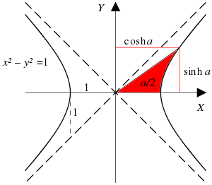
For a given value of a hyperbolic function, the corresponding inverse hyperbolic function provides the corresponding hyperbolic angle. The size of the hyperbolic angle is equal to the area of the corresponding hyperbolic sector of the hyperbola xy = 1, or twice the area of the corresponding sector of the unit hyperbola x² − y² = 1, just as a circular angle is twice the area of the circular sector of the unit circle. Some authors have called inverse hyperbolic functions "area functions" to realize the hyperbolic angles.^[1]^[2]^[3]^[4]^[5]^[6]^[7]^[8]

Hyperbolic functions and their inverses occur in many linear differential equations, for example the equation defining a catenary, of some cubic equations, in calculations of angles and distances in hyperbolic geometry and of Laplace's equation in Cartesian coordinates. Laplace's equations are important in many areas of physics, including electromagnetic theory, heat transfer, fluid dynamics, and special relativity.

Notation

The most common abbreviations and those specified by the ISO 80000-2 standard are ar- followed by the abbreviation of the corresponding hyperbolic function (arsinh, arcosh, etc.).

However, arc-, followed by the corresponding hyperbolic function (for example arcsinh, arccosh), is also commonly seen by analogy with the nomenclature for inverse trigonometric functions. The latter are misnomers, since the prefix arc is the abbreviation for arcus, while the prefix ar stands for area.^[9]^[10]^[11]

Other authors prefer to use the notation argsinh, argcosh, argtanh, and so on, where the prefix arg is the abbreviation of the Latin argumentum.^[12] In computer science this is often shortened to asinh.

The notation sinh⁻¹(x), cosh⁻¹(x), etc., is also used,^[13]^[14] despite the fact that care must be taken to avoid misinterpretations of the superscript −1 as a power as opposed to a shorthand to denote the inverse function (e.g., cosh⁻¹(x) versus cosh(x)⁻¹).

Definitions in terms of logarithms

As the hyperbolic functions are rational functions of $e x$ whose numerator and denominator are of degree at most two, these functions may be solved in terms of $e x$ , by using the quadratic formula; then, taking the natural logarithm gives the following expressions for the inverse hyperbolic functions.

For complex arguments, the inverse hyperbolic functions, the square root and the logarithm are multi-valued functions, and the equalities of the next subsections may be viewed as equalities of multi-valued functions.

For all inverse hyperbolic functions but the inverse hyperbolic cotangent and the inverse hyperbolic cosecant, the domain of the real function is connected.

Inverse hyperbolic sine

Inverse hyperbolic sine aka area hyperbolic sine (Latin: Area sinus hyperbolicus):

\operatorname {arsinh} x=\ln \left(x+{\sqrt {x^{2}+1}}\right)

The domain is the whole real line.

Inverse hyperbolic cosine

Inverse hyperbolic cosine aka area hyperbolic cosine (Latin: Area cosinus hyperbolicus):

\operatorname {arcosh} x=\ln \left(x+{\sqrt {x^{2}-1}}\right)

The domain is the closed interval $[1, +\infty )$ .

Inverse hyperbolic tangent

Inverse hyperbolic tangent aka area hyperbolic tangent (Latin: Area tangens hyperbolicus):

\operatorname {artanh} x={\frac {1}{2}}\ln \left({\frac {1+x}{1-x}}\right)

The domain is the open interval $(-1, 1)$ .

Inverse hyperbolic cotangent

Inverse hyperbolic cotangent aka area hyperbolic cotangent (Latin: Area cotangens hyperbolicus):

\operatorname {arcoth} x={\frac {1}{2}}\ln \left({\frac {x+1}{x-1}}\right)

The domain is the union of the open intervals $(-\infty, -1)$ and $(1, +\infty)$ .

Inverse hyperbolic secant

Inverse hyperbolic secant aka area hyperbolic secant (Latin: Area secans hyperbolicus):

\operatorname {arsech} x=\ln \left({\frac {1}{x}}+{\sqrt {{\frac {1}{x^{2}}}-1}}\right)=\ln \left({\frac {1+{\sqrt {1-x^{2}}}}{x}}\right)

The domain is the semi-open interval $(0, 1]$ .

Inverse hyperbolic cosecant

Inverse hyperbolic cosecant aka area hyperbolic cosecant (Latin: Area cosecans hyperbolicus):

\operatorname {arcsch} x=\ln \left({\frac {1}{x}}+{\sqrt {{\frac {1}{x^{2}}}+1}}\right)

The domain is the real line with 0 removed.

Addition formulae

\operatorname {arsinh} u\pm \operatorname {arsinh} v=\operatorname {arsinh} \left(u{\sqrt {1+v^{2}}}\pm v{\sqrt {1+u^{2}}}\right)

\operatorname {arcosh} u\pm \operatorname {arcosh} v=\operatorname {arcosh} \left(uv\pm {\sqrt {(u^{2}-1)(v^{2}-1)}}\right)

\operatorname {artanh} u\pm \operatorname {artanh} v=\operatorname {artanh} \left({\frac {u\pm v}{1\pm uv}}\right)

{\begin{aligned}\operatorname {arsinh} u+\operatorname {arcosh} v&=\operatorname {arsinh} \left(uv+{\sqrt {(1+u^{2})(v^{2}-1)}}\right)\\&=\operatorname {arcosh} \left(v{\sqrt {1+u^{2}}}+u{\sqrt {v^{2}-1}}\right)\end{aligned}}

Other identities

{\begin{aligned}2\operatorname {arcosh} x&=\operatorname {arcosh} (2x^{2}-1)&\quad {\hbox{ for }}x\geq 1\\4\operatorname {arcosh} x&=\operatorname {arcosh} (8x^{4}-8x^{2}+1)&\quad {\hbox{ for }}x\geq 1\\2\operatorname {arsinh} x&=\operatorname {arcosh} (2x^{2}+1)&\quad {\hbox{ for }}x\geq 0\\4\operatorname {arsinh} x&=\operatorname {arcosh} (8x^{4}+8x^{2}+1)&\quad {\hbox{ for }}x\geq 0\end{aligned}}

\ln(x)=\operatorname {arcosh} \left({\frac {x^{2}+1}{2x}}\right)=\operatorname {arsinh} \left({\frac {x^{2}-1}{2x}}\right)=\operatorname {artanh} \left({\frac {x^{2}-1}{x^{2}+1}}\right)

Composition of hyperbolic and inverse hyperbolic functions

{\begin{aligned}&\sinh(\operatorname {arcosh} x)={\sqrt {x^{2}-1}}\quad {\text{for}}\quad |x|>1\\&\sinh(\operatorname {artanh} x)={\frac {x}{\sqrt {1-x^{2}}}}\quad {\text{for}}\quad -1<x<1\\&\cosh(\operatorname {arsinh} x)={\sqrt {1+x^{2}}}\\&\cosh(\operatorname {artanh} x)={\frac {1}{\sqrt {1-x^{2}}}}\quad {\text{for}}\quad -1<x<1\\&\tanh(\operatorname {arsinh} x)={\frac {x}{\sqrt {1+x^{2}}}}\\&\tanh(\operatorname {arcosh} x)={\frac {\sqrt {x^{2}-1}}{x}}\quad {\text{for}}\quad |x|>1\end{aligned}}

Composition of inverse hyperbolic and trigonometric functions

\operatorname {arsinh} \left(\tan \alpha \right)=\operatorname {artanh} \left(\sin \alpha \right)=\ln \left({\frac {1+\sin \alpha }{\cos \alpha }}\right)=\pm \operatorname {arcosh} \left({\frac {1}{\cos \alpha }}\right)

\ln \left(\left|\tan \alpha \right|\right)=-\operatorname {artanh} \left(\cos 2\alpha \right)

^[15]

Conversions

\ln x=\operatorname {artanh} \left({\frac {x^{2}-1}{x^{2}+1}}\right)=\operatorname {arsinh} \left({\frac {x^{2}-1}{2x}}\right)=\pm \operatorname {arcosh} \left({\frac {x^{2}+1}{2x}}\right)

\operatorname {artanh} x=\operatorname {arsinh} \left({\frac {x}{\sqrt {1-x^{2}}}}\right)=\pm \operatorname {arcosh} \left({\frac {1}{\sqrt {1-x^{2}}}}\right)

\operatorname {arsinh} x=\operatorname {artanh} \left({\frac {x}{\sqrt {1+x^{2}}}}\right)=\pm \operatorname {arcosh} \left({\sqrt {1+x^{2}}}\right)

\operatorname {arcosh} x=\left|\operatorname {arsinh} \left({\sqrt {x^{2}-1}}\right)\right|=\left|\operatorname {artanh} \left({\frac {\sqrt {x^{2}-1}}{x}}\right)\right|

Derivatives

{\begin{aligned}{\frac {d}{dx}}\operatorname {arsinh} x&{}={\frac {1}{\sqrt {x^{2}+1}}},{\text{ for all real }}x\\{\frac {d}{dx}}\operatorname {arcosh} x&{}={\frac {1}{\sqrt {x^{2}-1}}},{\text{ for all real }}x>1\\{\frac {d}{dx}}\operatorname {artanh} x&{}={\frac {1}{1-x^{2}}},{\text{ for all real }}|x|<1\\{\frac {d}{dx}}\operatorname {arcoth} x&{}={\frac {1}{1-x^{2}}},{\text{ for all real }}|x|>1\\{\frac {d}{dx}}\operatorname {arsech} x&{}={\frac {-1}{x{\sqrt {1-x^{2}}}}},{\text{ for all real }}x\in (0,1)\\{\frac {d}{dx}}\operatorname {arcsch} x&{}={\frac {-1}{|x|{\sqrt {1+x^{2}}}}},{\text{ for all real }}x{\text{, except }}0\\\end{aligned}}

For an example differentiation: let θ = arsinh x, so (where sinh² θ = (sinh θ)²):

{\frac {d\,\operatorname {arsinh} x}{dx}}={\frac {d\theta }{d\sinh \theta }}={\frac {1}{\cosh \theta }}={\frac {1}{\sqrt {1+\sinh ^{2}\theta }}}={\frac {1}{\sqrt {1+x^{2}}}}.

Series expansions

Expansion series can be obtained for the above functions:

{\begin{aligned}\operatorname {arsinh} x&=x-\left({\frac {1}{2}}\right){\frac {x^{3}}{3}}+\left({\frac {1\cdot 3}{2\cdot 4}}\right){\frac {x^{5}}{5}}-\left({\frac {1\cdot 3\cdot 5}{2\cdot 4\cdot 6}}\right){\frac {x^{7}}{7}}\pm \cdots \\&=\sum _{n=0}^{\infty }\left({\frac {(-1)^{n}(2n)!}{2^{2n}(n!)^{2}}}\right){\frac {x^{2n+1}}{2n+1}},\qquad \left|x\right|<1\end{aligned}}

{\begin{aligned}\operatorname {arcosh} x&=\ln(2x)-\left(\left({\frac {1}{2}}\right){\frac {x^{-2}}{2}}+\left({\frac {1\cdot 3}{2\cdot 4}}\right){\frac {x^{-4}}{4}}+\left({\frac {1\cdot 3\cdot 5}{2\cdot 4\cdot 6}}\right){\frac {x^{-6}}{6}}+\cdots \right)\\&=\ln(2x)-\sum _{n=1}^{\infty }\left({\frac {(2n)!}{2^{2n}(n!)^{2}}}\right){\frac {x^{-2n}}{2n}},\qquad \left|x\right|>1\end{aligned}}

{\begin{aligned}\operatorname {artanh} x&=x+{\frac {x^{3}}{3}}+{\frac {x^{5}}{5}}+{\frac {x^{7}}{7}}+\cdots \\&=\sum _{n=0}^{\infty }{\frac {x^{2n+1}}{2n+1}},\qquad \left|x\right|<1\end{aligned}}

{\begin{aligned}\operatorname {arcsch} x=\operatorname {arsinh} {\frac {1}{x}}&=x^{-1}-\left({\frac {1}{2}}\right){\frac {x^{-3}}{3}}+\left({\frac {1\cdot 3}{2\cdot 4}}\right){\frac {x^{-5}}{5}}-\left({\frac {1\cdot 3\cdot 5}{2\cdot 4\cdot 6}}\right){\frac {x^{-7}}{7}}\pm \cdots \\&=\sum _{n=0}^{\infty }\left({\frac {(-1)^{n}(2n)!}{2^{2n}(n!)^{2}}}\right){\frac {x^{-(2n+1)}}{2n+1}},\qquad \left|x\right|>1\end{aligned}}

{\begin{aligned}\operatorname {arsech} x=\operatorname {arcosh} {\frac {1}{x}}&=\ln {\frac {2}{x}}-\left(\left({\frac {1}{2}}\right){\frac {x^{2}}{2}}+\left({\frac {1\cdot 3}{2\cdot 4}}\right){\frac {x^{4}}{4}}+\left({\frac {1\cdot 3\cdot 5}{2\cdot 4\cdot 6}}\right){\frac {x^{6}}{6}}+\cdots \right)\\&=\ln {\frac {2}{x}}-\sum _{n=1}^{\infty }\left({\frac {(2n)!}{2^{2n}(n!)^{2}}}\right){\frac {x^{2n}}{2n}},\qquad 0<x\leq 1\end{aligned}}

{\begin{aligned}\operatorname {arcoth} x=\operatorname {artanh} {\frac {1}{x}}&=x^{-1}+{\frac {x^{-3}}{3}}+{\frac {x^{-5}}{5}}+{\frac {x^{-7}}{7}}+\cdots \\&=\sum _{n=0}^{\infty }{\frac {x^{-(2n+1)}}{2n+1}},\qquad \left|x\right|>1\end{aligned}}

Asymptotic expansion for the arsinh x is given by

\operatorname {arsinh} x=\ln(2x)+\sum \limits _{n=1}^{\infty }{\left({-1}\right)^{n-1}{\frac {\left({2n-1}\right)!!}{2n\left({2n}\right)!!}}}{\frac {1}{x^{2n}}}

Principal values in the complex plane

As functions of a complex variable, inverse hyperbolic functions are multivalued functions that are analytic except at a finite number of points. For such a function, it is common to define a principal value, which is a single valued analytic function which coincides with one specific branch of the multivalued function over a domain consisting of the complex plane in which a finite number of arcs (usually half lines or line segments) have been removed. These arcs are called branch cuts. For specifying the branch, that is defining which value of the multivalued function is considered at each point, one generally define it at a particular point, and deduce the value everywhere in the domain of definition of the principal value by analytic continuation. When possible, it is better to define the principal value directly, without referring to analytic continuation.

For example, for the square root, the principal value is defined as the square root that has a positive real part. This defines a single valued analytic function, which is defined everywhere except for non-positive real values of the variables (where the two square roots have a zero real part). This principal value of the square root function is denoted ${\sqrt {x}}$ in what follows. Similarly, the principal value of the logarithm, denoted $\operatorname {Log}$ in what follows, is defined as the value for which the imaginary part as the smallest absolute value. It is defined everywhere except for non positive real values of the variable, for which two different values of the logarithm reach the minimum.

For all inverse hyperbolic functions, the principal value may be defined in terms of principal values of the square root and the logarithm function. However, in some cases, the formulas of § Definitions in terms of logarithms do not give a correct principal value, as giving a domain of definition which is too small and, in one case non-connected.

Principal value of the inverse hyperbolic sine

The principal value of the inverse hyperbolic sine is given by

\operatorname {arsinh} z=\operatorname {Log} (z+{\sqrt {z^{2}+1}}\,)\,.

The argument of the square root is a non-positive real number if and only if $z$ belongs to one of the intervals $[i, + i \infty)$ and $(- i \infty, - i]$ of the imaginary axis. If the argument of the logarithm is real, then it is positive. Thus this formula defines a principal value for arsinh with branch cuts $[i, + i \infty)$ and $(- i \infty, - i]$ . This is optimal, as the branch cuts must connect the singular points $i$ and $- i$ to the infinity.

Principal value of the inverse hyperbolic cosine

The formula for the inverse hyperbolic cosine given in § Inverse hyperbolic cosine is not convenient, as, with principal values of the logarithm and the square root, the principal value of arcosh would not be defined for imaginary $z$ . Thus the square root has to be factorized, leading to

\operatorname {arcosh} z=\operatorname {Log} (z+{\sqrt {z+1}}{\sqrt {z-1}}\,)\,.

The principal values of the square roots are both defined except if $z$ belongs to the real interval $(-\infty, 1]$ . If the argument of the logarithm is real, then $z$ is real and has the same sign. Thus, the above formula defines a principal value of arcosh outside the real interval $(-\infty, 1]$ , which is thus the unique branch cut.

Principal values of the inverse hyperbolic tangent and cotangent

The formulas given in § Definitions in terms of logarithms suggests

{\begin{aligned}\operatorname {artanh} z&={\frac {1}{2}}\operatorname {Log} \left({\frac {1+z}{1-z}}\right)\\\operatorname {arcoth} z&={\frac {1}{2}}\operatorname {Log} \left({\frac {z+1}{z-1}}\right)\end{aligned}}

for the definition of the principal values of the inverse hyperbolic tangent and cotangent. In these formulas, the argument of the logarithm is real if and only if $z$ is real. For artanh, this argument is in the real interval $(-\infty, 0]$ if $z$ belongs either to $(-\infty, -1]$ or to $[1, \infty)$ . For arcoth, the argument of the logarithm is in $(-\infty, 0]$ if and only if $z$ belongs to the real interval $[-1, 1]$ .

Therefore, these formulas define convenient principal values, for which the branch cuts are $(-\infty, -1]$ and $[1, \infty)$ for the inverse hyperbolic tangent, and $[-1, 1]$ for the inverse hyperbolic cotangent.

In view of a better numerical evaluation near the branch cuts, some authors use the following equivalent definition of the principal values, although the second one introduces a removable singularity at $z = 0$ .

{\begin{aligned}\operatorname {artanh} z&={\tfrac {1}{2}}\operatorname {Log} \left({1+z}\right)-{\tfrac {1}{2}}\operatorname {Log} \left({1-z}\right)\\\operatorname {arcoth} z&={\tfrac {1}{2}}\operatorname {Log} \left({1+{\frac {1}{z}}}\right)-{\tfrac {1}{2}}\operatorname {Log} \left({1-{\frac {1}{z}}}\right)\end{aligned}}

Principal value of the inverse hyperbolic cosecant

For the inverse hyperbolic cosecant, the principal value is defined as

\operatorname {arcsch} z=\operatorname {Log} \left({\frac {1}{z}}+{\sqrt {{\frac {1}{z^{2}}}+1}}\,\right)

.

It is defined when the arguments of the logarithm and the square root are not non-positive real numbers. The principal value of the square root is thus defined outside the interval $[- i, i]$ of the imaginary line. If the argument of the logarithm is real, then $z$ is a non-zero real number, and this implies that the argument of the logarithm is positive.

Thus the principal value is defined by the above formula outside the branch cut consisting of the interval $[- i, i]$ of the imaginary line.

For $z = 0$ , there is a singular point that is included in the branch cut.

Principal value of the inverse hyperbolic secant

Here, as in the case of the inverse hyperbolic cosine, we have to factorize the square root. This gives the principal value

\operatorname {arsech} z=\operatorname {Log} \left({\frac {1}{z}}+{\sqrt {{\frac {1}{z}}+1}}\,{\sqrt {{\frac {1}{z}}-1}}\right).

If the argument of a square root is real, then $z$ is real, and it follows that both principal values of square roots are defined except if $z$ is real and belongs to one of the intervals $(-\infty, 0]$ and $[1, +\infty)$ . If the argument of the logarithm is real and negative, then $z$ is also real and negative. It follows that the principal value of arsech is well defined by the above formula outside two branch cuts, the real intervals $(-\infty, 0]$ and $[1, +\infty)$ .

For $z = 0$ , there is a singular point that is included in one of the branch cuts.

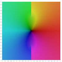
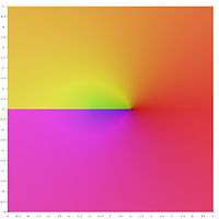
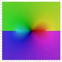
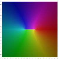
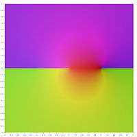
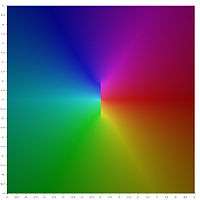
Graphical representation

In the following graphical representation of the principal values of the inverse hyperbolic functions, the branch cuts appear as discontinuities of the color. The fact that the whole branch cuts appear as discontinuities, shows that these principal values may not be extended into analytic functions defined over larger domains. In other words, the above defined branch cuts are minimal.

Square representing central portion of the complex z-plane painted in psychedelic colours

\operatorname {arsinh} (z)

\operatorname {arcosh} (z)

\operatorname {artanh} (z)

\operatorname {arcoth} (z)

\operatorname {arsech} (z)

\operatorname {arcsch} (z)

Inverse hyperbolic functions in the complex z-plane: the colour at each point in the plane represents the complex value of the respective function at that point

References

↑ Bronshtein, Ilja N.; Semendyayev, Konstantin A.; Musiol, Gerhard; Mühlig, Heiner (2007). "Chapter 2.10: Area Functions". Handbook of Mathematics (5 ed.). Springer-Verlag. p. 91. doi:10.1007/978-3-540-72122-2. ISBN 3-540-72121-5.
↑ Ebner, Dieter (2005-07-25). Preparatory Course in Mathematics (PDF) (6 ed.). Department of Physics, University of Konstanz. Archived (PDF) from the original on 2017-07-26. Retrieved 2017-07-26.
↑ Mejlbro, Leif (2006). Real Functions in One Variable – Calculus (PDF). 1a (1 ed.). Ventus Publishing ApS / Bookboon. ISBN 87-7681-117-4. Archived (PDF) from the original on 2017-07-26. Retrieved 2017-07-26.
↑ Mejlbro, Leif (2008). The Argument Principle and Many-valued Functions - Complex Functions Examples (PDF). c-9 (1 ed.). Ventus Publishing ApS / Bookboon. ISBN 978-87-7681-395-6. Archived (PDF) from the original on 2017-07-26. Retrieved 2017-07-26.
↑ Mejlbro, Leif (2010-11-11). Stability, Riemann Surfaces, Conformal Mappings - Complex Functions Theory (PDF). a-3 (1 ed.). Ventus Publishing ApS / Bookboon. ISBN 978-87-7681-702-2. ISBN 87-7681-702-4. Archived (PDF) from the original on 2017-07-26. Retrieved 2017-07-26.
↑ Durán, Mario (2012). Mathematical methods for wave propagation in science and engineering. 1: Fundamentals (1 ed.). Ediciones UC. p. 89. ISBN 978-956141314-6. ISBN 956141314-0.
↑ Weltner, Klaus; John, Sebastian; Weber, Wolfgang J.; Schuster, Peter; Grosjean, Jean (2014-06-27) [2009]. Mathematics for Physicists and Engineers: Fundamentals and Interactive Study Guide (2 ed.). Springer-Verlag. ISBN 978-364254124-7. ISBN 3642541240.
↑ Detlef Reimers http://tug.ctan.org/macros/latex/contrib/lapdf/fplot.pdf
↑ As stated by Jan Gullberg, Mathematics: From the Birth of Numbers (New York: W. W. Norton & Company, 1997), ISBN 0-393-04002-X, p. 539:
Another form of notation, arcsinh x, arccosh x, etc., is a practice to be condemned as these functions have nothing whatever to do with arc, but with area, as is demonstrated by their full Latin names,
arsinh area sinus hyperbolicus
arcosh area cosinus hyperbolicus, etc.
↑ As stated by Eberhard Zeidler, Wolfgang Hackbusch and Hans Rudolf Schwarz, translated by Bruce Hunt, Oxford Users' Guide to Mathematics (Oxford: Oxford University Press, 2004), ISBN 0-19-850763-1, Section 0.2.13: "The inverse hyperbolic functions", p. 68: "The Latin names for the inverse hyperbolic functions are area sinus hyperbolicus, area cosinus hyperbolicus, area tangens hyperbolicus and area cotangens hyperbolicus (of x). ..." This aforesaid reference uses the notations arsinh, arcosh, artanh, and arcoth for the respective inverse hyperbolic functions.
↑ As stated by Ilja N. Bronshtein, Konstantin A. Semendyayev, Gerhard Musiol and Heiner Mühlig, Handbook of Mathematics (Berlin: Springer-Verlag, 5th ed., 2007), ISBN 3-540-72121-5, doi:10.1007/978-3-540-72122-2, Section 2.10: "Area Functions", p. 91:
The area functions are the inverse functions of the hyperbolic functions, i.e., the inverse hyperbolic functions. The functions sinh x, tanh x, and coth x are strictly monotone, so they have unique inverses without any restriction; the function cosh x has two monotonic intervals so we can consider two inverse functions. The name area refers to the fact that the geometric definition of the functions is the area of certain hyperbolic sectors ...
↑ Bacon, Harold Maile (1942). Differential and Integral Calculus. McGraw-Hill. p. 203.
↑ Press, WH; Teukolsky, SA; Vetterling, WT; Flannery, BP (1992). "Section 5.6. Quadratic and Cubic Equations". Numerical Recipes in FORTRAN: The Art of Scientific Computing (2nd ed.). New York: Cambridge University Press. ISBN 0-521-43064-X.
↑ Woodhouse, N. M. J. (2003), Special Relativity, London: Springer, p. 71, ISBN 1-85233-426-6
↑ "Identities with inverse hyperbolic and trigonometric functions". math stackexchange. stackexchange. Retrieved 3 November 2016.

Herbert Busemann and Paul J. Kelly (1953) Projective Geometry and Projective Metrics, page 207, Academic Press.

External links

Hazewinkel, Michiel, ed. (2001) [1994], "Inverse hyperbolic functions", Encyclopedia of Mathematics, Springer Science+Business Media B.V. / Kluwer Academic Publishers, ISBN 978-1-55608-010-4
Inverse hyperbolic functions at MathWorld

This article is issued from Wikipedia. The text is licensed under Creative Commons - Attribution - Sharealike. Additional terms may apply for the media files.

[Bronshtein_2005-1] Bronshtein, Ilja N.; Semendyayev, Konstantin A.; Musiol, Gerhard; Mühlig, Heiner (2007). "Chapter 2.10: Area Functions". Handbook of Mathematics (5 ed.). Springer-Verlag. p. 91. doi:10.1007/978-3-540-72122-2. ISBN 3-540-72121-5.

[Ebner_2005-2] Ebner, Dieter (2005-07-25). Preparatory Course in Mathematics (PDF) (6 ed.). Department of Physics, University of Konstanz. Archived (PDF) from the original on 2017-07-26. Retrieved 2017-07-26.

[Mejlbro_2006-3] Mejlbro, Leif (2006). Real Functions in One Variable – Calculus (PDF). 1a (1 ed.). Ventus Publishing ApS / Bookboon. ISBN 87-7681-117-4. Archived (PDF) from the original on 2017-07-26. Retrieved 2017-07-26.

[Mejlbro_2008-4] Mejlbro, Leif (2008). The Argument Principle and Many-valued Functions - Complex Functions Examples (PDF). c-9 (1 ed.). Ventus Publishing ApS / Bookboon. ISBN 978-87-7681-395-6. Archived (PDF) from the original on 2017-07-26. Retrieved 2017-07-26.

[Mejlbro_2010-5] Mejlbro, Leif (2010-11-11). Stability, Riemann Surfaces, Conformal Mappings - Complex Functions Theory (PDF). a-3 (1 ed.). Ventus Publishing ApS / Bookboon. ISBN 978-87-7681-702-2. ISBN 87-7681-702-4. Archived (PDF) from the original on 2017-07-26. Retrieved 2017-07-26.

[Duran_2012-6] Durán, Mario (2012). Mathematical methods for wave propagation in science and engineering. 1: Fundamentals (1 ed.). Ediciones UC. p. 89. ISBN 978-956141314-6. ISBN 956141314-0.

[Weltner_2014-7] Weltner, Klaus; John, Sebastian; Weber, Wolfgang J.; Schuster, Peter; Grosjean, Jean (2014-06-27) [2009]. Mathematics for Physicists and Engineers: Fundamentals and Interactive Study Guide (2 ed.). Springer-Verlag. ISBN 978-364254124-7. ISBN 3642541240.

[Reimers_Lapdf-8] Detlef Reimers http://tug.ctan.org/macros/latex/contrib/lapdf/fplot.pdf

[Gullberg1997-9] As stated by Jan Gullberg, Mathematics: From the Birth of Numbers (New York: W. W. Norton & Company, 1997), ISBN 0-393-04002-X, p. 539:
Another form of notation, arcsinh x, arccosh x, etc., is a practice to be condemned as these functions have nothing whatever to do with arc, but with area, as is demonstrated by their full Latin names,
arsinh area sinus hyperbolicus
arcosh area cosinus hyperbolicus, etc.

[ZeidlerEtAl2004-10] As stated by Eberhard Zeidler, Wolfgang Hackbusch and Hans Rudolf Schwarz, translated by Bruce Hunt, Oxford Users' Guide to Mathematics (Oxford: Oxford University Press, 2004), ISBN 0-19-850763-1, Section 0.2.13: "The inverse hyperbolic functions", p. 68: "The Latin names for the inverse hyperbolic functions are area sinus hyperbolicus, area cosinus hyperbolicus, area tangens hyperbolicus and area cotangens hyperbolicus (of x). ..." This aforesaid reference uses the notations arsinh, arcosh, artanh, and arcoth for the respective inverse hyperbolic functions.

[BronshteinEtAl2007-11] As stated by Ilja N. Bronshtein, Konstantin A. Semendyayev, Gerhard Musiol and Heiner Mühlig, Handbook of Mathematics (Berlin: Springer-Verlag, 5th ed., 2007), ISBN 3-540-72121-5, doi:10.1007/978-3-540-72122-2, Section 2.10: "Area Functions", p. 91:
The area functions are the inverse functions of the hyperbolic functions, i.e., the inverse hyperbolic functions. The functions sinh x, tanh x, and coth x are strictly monotone, so they have unique inverses without any restriction; the function cosh x has two monotonic intervals so we can consider two inverse functions. The name area refers to the fact that the geometric definition of the functions is the area of certain hyperbolic sectors ...

[12] Bacon, Harold Maile (1942). Differential and Integral Calculus. McGraw-Hill. p. 203.

[Press1992-13] Press, WH; Teukolsky, SA; Vetterling, WT; Flannery, BP (1992). "Section 5.6. Quadratic and Cubic Equations". Numerical Recipes in FORTRAN: The Art of Scientific Computing (2nd ed.). New York: Cambridge University Press. ISBN 0-521-43064-X.

[14] Woodhouse, N. M. J. (2003), Special Relativity, London: Springer, p. 71, ISBN 1-85233-426-6

[15] "Identities with inverse hyperbolic and trigonometric functions". math stackexchange. stackexchange. Retrieved 3 November 2016.