Hyperbolic angle

The hyperbolic angle u is a real number that is the argument of the hyperbolic functions sinh and cosh. It determines a hyperbolic sector (red) that has area u (defined to be negative for the case shown here because x < 1 at the point on the hyperbola). The legs of the hyperbolic triangle (yellow) are proportional to sinh(u) and cosh(u).

Top: Positive and negative hyperbolic angles. Bottom: The difference between the two positive angles is shown as Δu = u₂ − u₁.

In mathematics, a hyperbolic angle is a geometric figure that defines a section of a hyperbola. The relationship of a hyperbolic angle to a hyperbola parallels the relationship of an "ordinary" angle to a circle.

Hyperbolic angle is defined in terms of the "standard" rectangular hyperbola: y = 1/x, for positive x. It can be described as the angle subtended at the origin by a given interval on the hyperbola, while its magnitude is defined as the magnitude of the area so subtended - that is, the area bounded on two sides by rays from the origin to the endpoints of the interval and on the third side by the curve of the interval itself.

Hyperbolic angle is used as the independent variable for the hyperbolic functions sinh, cosh, and tanh, because these functions may be premised on hyperbolic analogies to the corresponding circular trigonometric functions by regarding a hyperbolic angle as defining a hyperbolic triangle. The parameter thus becomes one of the most useful in the calculus of real variables.

Definition

We consider the rectangular hyperbola $\textstyle \{(x,{\frac {1}{x}}):x>0\}$ , and (by convention) pay particular attention to the branch $x>1$ .

We first define:

The hyperbolic angle in standard position is the angle at $(0,0)$ between the ray to $(1,1)$ and the ray to $\textstyle (x,{\frac {1}{x}})$ , where $x>1$ .
The magnitude of this angle is the area of the corresponding hyperbolic sector, which turns out to be $\operatorname {ln} x$ .

Note that, because of the role played by the natural logarithm:

Unlike the circular angle, the hyperbolic angle is unbounded (because $\operatorname {ln} x$ is unbounded); this is related to the fact that the harmonic series is unbounded.
The formula for the magnitude of the angle suggests that, for $0 < x < 1$ , the hyperbolic angle should be negative. This reflects the fact that, as defined, the angle is directed.

Finally, we extend the definition of hyperbolic angle to that subtended by any interval on the hyperbola. Suppose $a, b, c, d$ are real numbers such that $ab=cd=1$ and $c>a>1$ , so that $(a,b)$ and $(c,d)$ are points on the hyperbola $xy=1$ and determine an interval on it. Then the squeeze mapping $\textstyle f:(x,y)\to (bx,ay)$ maps the angle $\angle \!\left((a,b),(0,0),(c,d)\right)$ to the standard position angle $\angle \!\left((1,1),(0,0),(bc,ad)\right)$ . By the result of Gregoire de Saint-Vincent, the hyperbolic sectors determined by these angles have the same area, which is taken to be the magnitude of the angle. This magnitude is $\operatorname {ln} {(bc)}=\operatorname {ln} (c/a)=\operatorname {ln} c-\operatorname {ln} a$ .

Comparison with circular angle

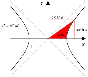
The unit hyperbola has a sector with an area half of the hyperbolic angle

Circular vs. hyperbolic angle

A unit circle $x^2 + y^2 = 1$ has a circular sector with an area half of the circular angle in radians. Analogously, a unit hyperbola $x^{2}-y^{2}=1$ has a hyperbolic sector with an area half of the hyperbolic angle.

There is also a projective resolution between circular and hyperbolic cases: both curves are conic sections, and hence are treated as projective ranges in projective geometry. Given an origin point on one of these ranges, other points correspond to angles. The idea of addition of angles, basic to science, corresponds to addition of points on one of these ranges as follows:

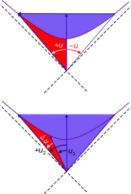
Circular angles can be characterised geometrically by the property that if two chords P₀P₁ and P₀P₂ subtend angles L₁ and L₂ at the centre of a circle, their sum L₁ + L₂ is the angle subtended by a chord PQ, where PQ is required to be parallel to P₁P₂.

The same construction can also be applied to the hyperbola. If P₀ is taken to be the point (1, 1), P₁ the point (x₁, 1/x₁), and P₂ the point (x₂, 1/x₂), then the parallel condition requires that Q be the point (x₁x₂, 1/x₁1/x₂). It thus makes sense to define the hyperbolic angle from P₀ to an arbitrary point on the curve as a logarithmic function of the point's value of x.^[1]^[2]

Whereas in Euclidean geometry moving steadily in an orthogonal direction to a ray from the origin traces out a circle, in a pseudo-Euclidean plane steadily moving orthogonally to a ray from the origin traces out a hyperbola. In Euclidean space, the multiple of a given angle traces equal distances around a circle while it traces exponential distances upon the hyperbolic line.^[3]

Both circular and hyperbolic angle provide instances of an invariant measure. Arcs with an angular magnitude on a circle generate a measure on certain measurable sets on the circle whose magnitude does not vary as the circle turns or rotates. For the hyperbola the turning is by squeeze mapping, and the hyperbolic angle magnitudes stay the same when the plane is squeezed by a mapping

(x, y) ↦ (rx, y / r), with r > 0 .

History

The quadrature of the hyperbola is the evaluation of the area of a hyperbolic sector. It can be shown to be equal to the corresponding area against an asymptote. The quadrature was first accomplished by Gregoire de Saint-Vincent in 1647 in his momentous Opus geometricum quadrature circuli et sectionum coni. As expressed by a historian,

[He made the] quadrature of a hyperbola to its asymptotes, and showed that as the area increased in arithmetic series the abscissas increased in geometric series.^[4]

A. A. de Sarasa interpreted the quadrature as a logarithm and thus the geometrically defined natural logarithm (or "hyperbolic logarithm") is understood as the area under y = 1/x to the right of x = 1. As an example of a transcendental function, the logarithm is more familiar than its motivator, the hyperbolic angle. Nevertheless, the hyperbolic angle plays a role when the theorem of Saint-Vincent is advanced with squeeze mapping.

Circular trigonometry was extended to the hyperbola by Augustus De Morgan in his textbook Trigonometry and Double Algebra.^[5] In 1878 W.K. Clifford used the hyperbolic angle to parametrize a unit hyperbola, describing it as "quasi-harmonic motion".

In 1894 Alexander Macfarlane circulated his essay "The Imaginary of Algebra", which used hyperbolic angles to generate hyperbolic versors, in his book Papers on Space Analysis.^[6] The following year Bulletin of the American Mathematical Society published Mellen W. Haskell's outline of the hyperbolic functions.^[7]

When Ludwik Silberstein penned his popular 1914 textbook on the new theory of relativity, he used the rapidity concept based on hyperbolic angle a, where tanh a = v/c, the ratio of velocity v to the speed of light. He wrote:

It seems worth mentioning that to unit rapidity corresponds a huge velocity, amounting to 3/4 of the velocity of light; more accurately we have v = (.7616)c for a = 1.

[...] the rapidity a = 1, [...] consequently will represent the velocity .76 c which is a little above the velocity of light in water.

Silberstein also uses Lobachevsky's concept of angle of parallelism Π(a) to obtain cos Π(a) = v/c.^[8]

Imaginary circular angle

The hyperbolic angle is often presented as if it were an imaginary number. Thus, if x is a real number and i² = −1, then

\cos(ix)=\cosh(x)\quad {\text{and}}\quad \sin(ix)=i\sinh(x)

so that the hyperbolic functions cosh and sinh can be presented through the circular functions. But these identities do not arise from a circle or rotation, rather they can be understood in terms of infinite series. In particular, the one expressing the exponential function ( $e^{x}=\cosh x+\sinh x\!$ ) consists of even and odd terms, the former comprise the cosh function ( $\textstyle \cosh x=\sum _{{n=0}}^{\infty }{\frac {x^{{2n}}}{(2n)!}}$ ), the latter the sinh function ( $\textstyle \sinh x=\sum _{{n=0}}^{\infty }{\frac {x^{{2n+1}}}{(2n+1)!}}$ ). The infinite series for cosine is derived from cosh by turning it into an alternating series, and the series for sine comes from making sinh into an alternating series. The above identities use the number i to remove the alternating factor (−1)ⁿ from terms of the series to restore the full halves of the exponential series. Nevertheless, in the theory of holomorphic functions, the hyperbolic sine and cosine functions are incorporated into the complex sine and cosine functions.

Notes

↑ Bjørn Felsager, Through the Looking Glass – A glimpse of Euclid's twin geometry, the Minkowski geometry, ICME-10 Copenhagen 2004; p.14. See also example sheets exploring Minkowskian parallels of some standard Euclidean results
↑ Viktor Prasolov and Yuri Solovyev (1997) Elliptic Functions and Elliptic Integrals, page 1, Translations of Mathematical Monographs volume 170, American Mathematical Society
↑ Hyperbolic Geometry pp 5–6, Fig 15.1
↑ David Eugene Smith (1925) History of Mathematics, pp. 424,5 v. 1
↑ Augustus De Morgan (1849) Trigonometry and Double Algebra, Chapter VI: "On the connection of common and hyperbolic trigonometry"
↑ Alexander Macfarlane(1894) Papers on Space Analysis, B. Westerman, New York
↑ Mellen W. Haskell (1895) On the introduction of the notion of hyperbolic functions Bulletin of the American Mathematical Society 1(6):155–9
↑ Ludwik Silberstein (1914) Theory of Relativity, Cambridge University Press, pp. 180–1

References

Janet Heine Barnett (2004) "Enter, stage center: the early drama of the hyperbolic functions", available in (a) Mathematics Magazine 77(1):15–30 or (b) chapter 7 of Euler at 300, RE Bradley, LA D'Antonio, CE Sandifer editors, Mathematical Association of America ISBN 0-88385-565-8 .
Arthur Kennelly (1912) Application of hyperbolic functions to electrical engineering problems
William Mueller, Exploring Precalculus, § The Number e, Hyperbolic Trigonometry.
John Stillwell (1998) Numbers and Geometry exercise 9.5.3, p. 298, Springer-Verlag ISBN 0-387-98289-2.

This article is issued from Wikipedia. The text is licensed under Creative Commons - Attribution - Sharealike. Additional terms may apply for the media files.

[1] Bjørn Felsager, Through the Looking Glass – A glimpse of Euclid's twin geometry, the Minkowski geometry, ICME-10 Copenhagen 2004; p.14. See also example sheets exploring Minkowskian parallels of some standard Euclidean results

[2] Viktor Prasolov and Yuri Solovyev (1997) Elliptic Functions and Elliptic Integrals, page 1, Translations of Mathematical Monographs volume 170, American Mathematical Society

[3] Hyperbolic Geometry pp 5–6, Fig 15.1

[4] David Eugene Smith (1925) History of Mathematics, pp. 424,5 v. 1

[5] Augustus De Morgan (1849) Trigonometry and Double Algebra, Chapter VI: "On the connection of common and hyperbolic trigonometry"

[6] Alexander Macfarlane(1894) Papers on Space Analysis, B. Westerman, New York

[7] Mellen W. Haskell (1895) On the introduction of the notion of hyperbolic functions Bulletin of the American Mathematical Society 1(6):155–9

[8] Ludwik Silberstein (1914) Theory of Relativity, Cambridge University Press, pp. 180–1